摘要
本文介绍了一个使用R语言重新绘制MaxEnt模型响应曲线的方法,旨在解决原版MaxEnt输出图形美观度不足且非矢量格式的问题。该方法通过R脚本实现以下功能:
- 自动读取MaxEnt输出数据(包括plots目录中的响应曲线数据和maxentResults.csv中的阈值数据)
- 支持连续变量和分类变量的自动识别与处理
- 为连续变量计算误差带(基于10次重复运行结果)
- 在图中标注两条重要阈值线(最大训练灵敏度+特异度阈值和平衡训练阈值)
- 输出PNG、PDF和SVG三种格式的矢量图形,便于在PPT中编辑
使用前需要修改脚本中的输入输出目录路径,并可根据需要调整物种名称(默认"MF")和输出格式(cloglog/logistic)。脚本还包含中文变量标签的自动转换功能,特别适合处理包含中文环境变量的情况。最终输出为分页排列的响应曲线图(每页3×4布局),同时生成变量汇总表记录各变量的统计信息。
问题说明
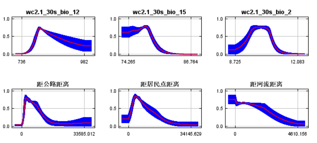
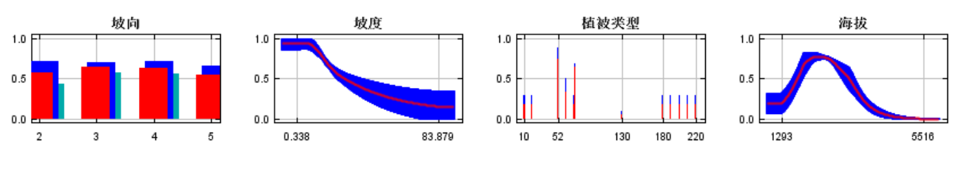
使用MaxEntVersion 3.4.1建模后会输出响应曲线图,但是这些图不太美观 ,而且不是矢量图无法随意调整,因此可以使用R语言对结果数据重新作图。
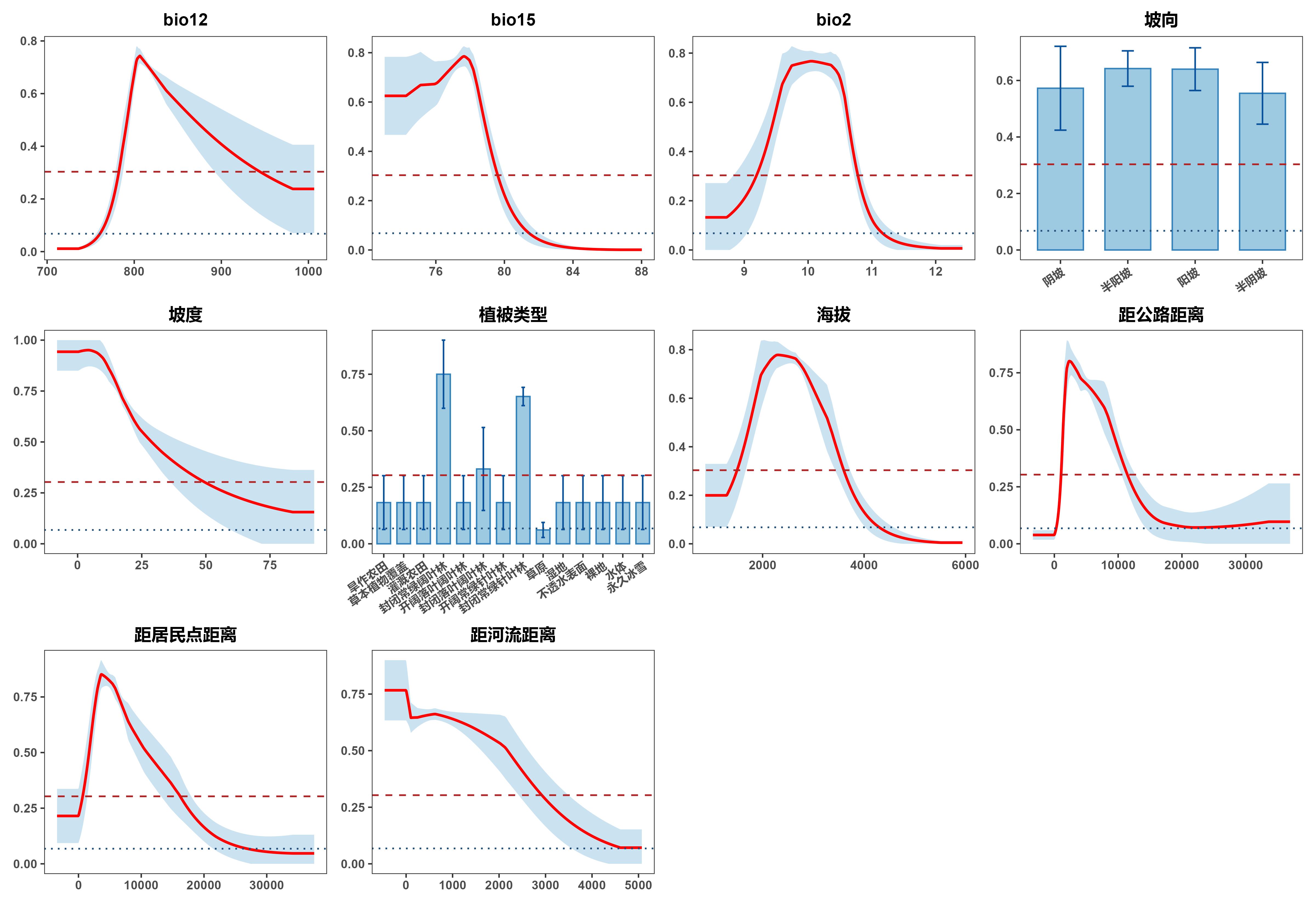
下面是R语言作图结果,后续可以将svg文件拖入PPT中,就可以随意修改任意要素了。
代码
下面是R语言的代码,需要注意以下几点:(比如我的建模物种名称为MF,所以大部分数据名称都是MF开头)根据自己数据情况修改
1.数据目录。
在代码42行选择你的maxent输出的plots目录,比如我的就是E:/paper3/maxent5/MF/plots。
在43行选择你的maxentResults.csv的目录,比如我的就是E:/paper3/maxent5/MF/maxentResults.csv
在44行选择你想要输出的文件夹,比如我的就是E:/paper3/maxent5/curves/MF_curve,先创建E:/paper3/maxent5/curves文件夹,r代码结果会在curves文件夹里自动创建一个名为MF_curve的文件夹。输出结果包括png、PDF和svg文件。
2.曲线和误差带使用的数据。
使用输出结果的plots文件夹,代码会自动检索环境变量文件,遵循的规则是"MF_因子_only.dat"。如果建模时重复了10次,那么就会以平均值那个数据作为主线,其他数据计算误差带。
3.两条阈值数据。
使用的是输出结果的名为maxentResults.csv的Excel数据,代码会自动检索行名称为"MF (average)",列名为"Maximum training sensitivity plus specificity Cloglog threshold",
"Balance training omission, predicted area and threshold value Cloglog threshold"。这里的"Cloglog"表示建模时候选择的Output format,如果选择的是logistic就把代码改为"Maximum training sensitivity plus specificity logistic threshold",
"Balance training omission, predicted area and threshold value logistic threshold"。
4.环境变量名称修改。
代码会自动识别连续变量和分类变量并相应作图,无需修改。坡向和植被类型的名称都从代号对应修改为了中文,在56行。气候变量因为我直接使用原始名称建模wc2.1_30s_bio_12,所以加一步全部简化为bio12,在154行,如果建模时候的名称没问题就不用管。
R
# =========================================================
# MaxEnt 响应曲线总图绘制脚本(修正版:连续变量插值后计算误差带)
# 输入目录: E:/paper3/maxent5/MF/plots
# 阈值文件: E:/paper3/maxent5/MF/maxentResults.csv
# 输出目录: E:/paper3/maxent5/curves/MF_curve
# =========================================================

rm(list = ls())
gc()

# -----------------------------
# 1. 加载包
# -----------------------------
pkg <- c("ggplot2", "dplyr", "stringr", "purrr", "patchwork", "svglite")
need <- pkg[!pkg %in% installed.packages()[, "Package"]]
if (length(need) > 0) install.packages(need)

library(ggplot2)
library(dplyr)
library(stringr)
library(purrr)
library(patchwork)
library(svglite)
# -----------------------------
# 字体设置(Windows)
# -----------------------------
windowsFonts(
  SimSun  = windowsFont("SimSun"),
  TimesNR = windowsFont("Times New Roman")
)

pick_family <- function(x) {
  if (stringr::str_detect(x, "[\u4e00-\u9fa5]")) {
    return("SimSun")
  } else {
    return("TimesNR")
  }
}
# -----------------------------
# 2. 路径设置
# -----------------------------
input_dir   <- "E:/paper3/maxent5/MF/plots"
result_file <- "E:/paper3/maxent5/MF/maxentResults.csv"
out_dir     <- "E:/paper3/maxent5/curves/MF_curve"

if (!dir.exists(input_dir)) stop(paste0("输入数据目录不存在:", input_dir))
if (!file.exists(result_file)) stop(paste0("maxentResults.csv 不存在:", result_file))
if (!dir.exists(out_dir)) dir.create(out_dir, recursive = TRUE)

# -----------------------------
# 3. 分类变量清单
# -----------------------------
manual_categorical_vars <- c("坡向", "植被类型", "土地利用类型")

# -----------------------------
# 4. 标签映射
# -----------------------------
aspect_labels <- c(
  "1" = "平地",
  "2" = "阴坡",
  "3" = "半阳坡",
  "4" = "阳坡",
  "5" = "半阴坡"
)

vegetation_labels <- c(
  "10"  = "旱作农田",
  "11"  = "草本植物覆盖",
  "20"  = "灌溉农田",
  "51"  = "开阔常绿阔叶林",
  "52"  = "封闭常绿阔叶林",
  "61"  = "开阔落叶阔叶林",
  "62"  = "封闭落叶阔叶林",
  "71"  = "开阔常绿针叶林",
  "72"  = "封闭常绿针叶林",
  "121" = "常绿灌木林",
  "122" = "落叶灌木林",
  "130" = "草原",
  "150" = "稀疏植被",
  "180" = "湿地",
  "190" = "不透水表面",
  "200" = "裸地",
  "201" = "牢固的裸地",
  "202" = "松散的裸地",
  "210" = "水体",
  "220" = "永久冰雪"
)

# -----------------------------
# 5. 安全读取 dat 文件
# -----------------------------
read_dat_safely <- function(file) {
  encodings <- c("UTF-8", "GB18030", "GBK", "CP936")

  for (enc in encodings) {
    dat <- tryCatch(
      read.csv(file, fileEncoding = enc, stringsAsFactors = FALSE),
      error = function(e) NULL
    )

    if (!is.null(dat) && ncol(dat) >= 3) {
      names(dat)[1:3] <- c("variable", "x", "y")
      dat$x <- suppressWarnings(as.numeric(dat$x))
      dat$y <- suppressWarnings(as.numeric(dat$y))
      dat <- dat[!is.na(dat$x) & !is.na(dat$y), ]
      if (nrow(dat) > 0) return(dat)
    }
  }

  stop(paste("无法读取文件:", file))
}

# -----------------------------
# 6. 解析文件名
# 支持:
#   MF_坡向_only.dat
#   MF_0_坡向_only.dat
#   MF_0_wc2.1_30s_bio_12_only.dat
# -----------------------------
parse_file_info <- function(file) {
  nm <- tools::file_path_sans_ext(basename(file))
  parts <- strsplit(nm, "_", fixed = TRUE)[[1]]

  if (length(parts) < 3) {
    return(data.frame(
      file = file,
      prefix = NA_character_,
      replicate = NA_integer_,
      variable_name_raw = NA_character_,
      stringsAsFactors = FALSE
    ))
  }

  if (grepl("^[0-9]+$", parts[2])) {
    prefix <- parts[1]
    replicate <- as.integer(parts[2])
    variable_name_raw <- paste(parts[3:(length(parts) - 1)], collapse = "_")
  } else {
    prefix <- parts[1]
    replicate <- NA_integer_
    variable_name_raw <- paste(parts[2:(length(parts) - 1)], collapse = "_")
  }

  data.frame(
    file = file,
    prefix = prefix,
    replicate = replicate,
    variable_name_raw = variable_name_raw,
    stringsAsFactors = FALSE
  )
}

# -----------------------------
# 7. 变量名美化
# wc2.1_30s_bio_12 -> bio12
# -----------------------------
pretty_var_name <- function(x) {
  x <- str_trim(x)

  if (str_detect(x, "^wc2\\.1_30s_bio_\\d+$")) {
    num <- str_extract(x, "\\d+$")
    return(paste0("bio", num))
  }

  return(x)
}

# -----------------------------
# 8. 判断变量类型
# -----------------------------
guess_var_type <- function(x, var_name = NULL) {
  if (!is.null(var_name) && var_name %in% manual_categorical_vars) {
    return("categorical")
  }

  ux <- sort(unique(x))
  is_integer_like <- all(abs(ux - round(ux)) < 1e-8)

  if (length(ux) <= 30 && is_integer_like) {
    return("categorical")
  } else {
    return("continuous")
  }
}

# -----------------------------
# 9. 精确读取阈值
# 行名: MF (average)
# -----------------------------
read_thresholds_exact <- function(result_file, row_name = "MF (average)") {
  res <- read.csv(result_file, stringsAsFactors = FALSE, check.names = FALSE)

  needed_cols <- c(
    "Maximum training sensitivity plus specificity Cloglog threshold",
    "Balance training omission, predicted area and threshold value Cloglog threshold"
  )

  missing_cols <- needed_cols[!needed_cols %in% names(res)]
  if (length(missing_cols) > 0) {
    stop(
      paste0(
        "maxentResults.csv 中缺少以下列:\n",
        paste(missing_cols, collapse = "\n")
      )
    )
  }

  char_cols <- sapply(res, function(z) is.character(z) || is.factor(z))
  if (!any(char_cols)) {
    stop("maxentResults.csv 中未找到字符列,无法识别 'MF (average)'。")
  }

  row_mask <- apply(res[, char_cols, drop = FALSE], 1, function(r) {
    any(trimws(as.character(r)) == row_name)
  })

  if (!any(row_mask)) {
    stop("未在 maxentResults.csv 中找到行名:MF (average)")
  }

  target_row <- res[row_mask, , drop = FALSE][1, ]

  mtss_val <- suppressWarnings(as.numeric(
    target_row[["Maximum training sensitivity plus specificity Cloglog threshold"]]
  ))

  btpt_val <- suppressWarnings(as.numeric(
    target_row[["Balance training omission, predicted area and threshold value Cloglog threshold"]]
  ))

  if (is.na(mtss_val) || is.na(btpt_val)) {
    stop("阈值读取到了,但转换为数值失败。")
  }

  list(
    mtss = mtss_val,
    btpt = btpt_val,
    row_name = row_name
  )
}

# -----------------------------
# 10. 分类变量中文标签
# -----------------------------
recode_categorical_labels <- function(plot_dat, var_name) {
  plot_dat <- plot_dat %>% arrange(x)

  if (var_name == "坡向") {
    x_chr <- as.character(plot_dat$x)
    lbls <- ifelse(x_chr %in% names(aspect_labels), aspect_labels[x_chr], x_chr)
    plot_dat$x_fac <- factor(lbls, levels = lbls)
    return(plot_dat)
  }

  if (var_name %in% c("植被类型", "土地利用类型")) {
    x_chr <- as.character(plot_dat$x)
    lbls <- ifelse(x_chr %in% names(vegetation_labels), vegetation_labels[x_chr], x_chr)
    plot_dat$x_fac <- factor(lbls, levels = lbls)
    return(plot_dat)
  }

  plot_dat$x_fac <- factor(plot_dat$x, levels = unique(plot_dat$x))
  plot_dat
}

# -----------------------------
# 11. 连续变量:把每次重复插值到参考 x 网格
# -----------------------------
interp_one_rep <- function(df_rep, ref_x) {
  df_rep <- df_rep %>%
    arrange(x) %>%
    group_by(x) %>%
    summarise(y = mean(y, na.rm = TRUE), .groups = "drop")

  if (nrow(df_rep) < 2) {
    return(rep(NA_real_, length(ref_x)))
  }

  approx(
    x = df_rep$x,
    y = df_rep$y,
    xout = ref_x,
    method = "linear",
    ties = mean,
    rule = 2
  )$y
}

# -----------------------------
# 12. 构建单变量绘图数据
# 关键:连续变量用插值后的重复曲线算 sd
# -----------------------------
build_plot_data <- function(var_name_raw, var_name_show, info_df) {
  sub_info <- info_df %>% filter(variable_name_raw == var_name_raw)

  avg_info <- sub_info %>% filter(is.na(replicate))
  rep_info <- sub_info %>% filter(!is.na(replicate))

  avg_dat <- NULL
  if (nrow(avg_info) >= 1) {
    avg_dat <- read_dat_safely(avg_info$file[1]) %>%
      select(x, y) %>%
      arrange(x)
  }

  rep_dat <- NULL
  if (nrow(rep_info) >= 1) {
    rep_dat <- map2_dfr(rep_info$file, rep_info$replicate, function(f, r) {
      d <- read_dat_safely(f)
      d$replicate <- r
      d %>% select(x, y, replicate)
    })
  }

  if (is.null(avg_dat) && is.null(rep_dat)) {
    stop(paste0("变量 ", var_name_raw, " 没有可用数据。"))
  }

  # 没有平均文件时,用重复结果生成参考网格
  if (is.null(avg_dat) && !is.null(rep_dat)) {
    avg_dat <- rep_dat %>%
      group_by(x) %>%
      summarise(y = mean(y, na.rm = TRUE), .groups = "drop") %>%
      arrange(x)
  }

  var_type <- guess_var_type(avg_dat$x, var_name_show)

  # -------------------------
  # 连续变量:插值到 avg_dat$x
  # -------------------------
  if (var_type == "continuous") {
    ref_x <- avg_dat$x

    if (!is.null(rep_dat) && n_distinct(rep_dat$replicate) >= 2) {
      rep_list <- split(rep_dat, rep_dat$replicate)
      interp_mat <- sapply(rep_list, function(df) interp_one_rep(df, ref_x))

      # 如果只有一个重复,sapply 可能变向量
      if (is.null(dim(interp_mat))) {
        interp_mat <- matrix(interp_mat, ncol = 1)
      }

      mean_y <- rowMeans(interp_mat, na.rm = TRUE)
      sd_y   <- apply(interp_mat, 1, sd, na.rm = TRUE)

      # 若某行全 NA,sd 会是 NA;这里保留即可
      plot_dat <- data.frame(
        x = ref_x,
        mean_y = mean_y,
        sd_y = sd_y,
        n_rep = ncol(interp_mat)
      )
    } else {
      plot_dat <- avg_dat %>%
        transmute(
          x = x,
          mean_y = y,
          sd_y = NA_real_,
          n_rep = ifelse(is.null(rep_dat), 0L, dplyr::n_distinct(rep_dat$replicate))
        )
    }

  } else {
    # -------------------------
    # 分类变量:直接按 x 汇总
    # -------------------------
    if (!is.null(rep_dat) && n_distinct(rep_dat$replicate) >= 2) {
      stat_dat <- rep_dat %>%
        group_by(x) %>%
        summarise(
          mean_y = mean(y, na.rm = TRUE),
          sd_y   = sd(y, na.rm = TRUE),
          n_rep  = n_distinct(replicate),
          .groups = "drop"
        ) %>%
        arrange(x)
      plot_dat <- stat_dat
    } else {
      plot_dat <- avg_dat %>%
        transmute(
          x = x,
          mean_y = y,
          sd_y = NA_real_,
          n_rep = ifelse(is.null(rep_dat), 0L, dplyr::n_distinct(rep_dat$replicate))
        )
    }
  }

  plot_dat <- plot_dat %>%
    mutate(
      ymin = ifelse(is.na(sd_y), NA_real_, pmax(mean_y - sd_y, 0)),
      ymax = ifelse(is.na(sd_y), NA_real_, pmin(mean_y + sd_y, 1))
    ) %>%
    arrange(x)

  list(
    plot_dat = plot_dat,
    var_type = var_type,
    rep_files_n = ifelse(is.null(rep_dat), 0L, dplyr::n_distinct(rep_dat$replicate)),
    sd_available = any(!is.na(plot_dat$sd_y)),
    sd_max = suppressWarnings(max(plot_dat$sd_y, na.rm = TRUE))
  )
}

# -----------------------------
# 13. 单变量生成子图
# -----------------------------
make_one_plot <- function(var_name_raw, var_name_show, info_df, mtss, btpt) {
  built <- build_plot_data(var_name_raw, var_name_show, info_df)
  plot_dat <- built$plot_dat
  var_type <- built$var_type

  title_family <- pick_family(var_name_show)

  if (var_type == "continuous") {
    p <- ggplot(plot_dat, aes(x = x, y = mean_y)) +
      geom_ribbon(
        aes(ymin = ymin, ymax = ymax),
        fill = "#6BAED6", alpha = 0.35, na.rm = TRUE
      ) +
      geom_line(color = "red", linewidth = 1.1) +
      geom_hline(yintercept = mtss, linetype = "dashed", color = "#B22222", linewidth = 0.7) +
      geom_hline(yintercept = btpt, linetype = "dotted", color = "#1F4E79", linewidth = 0.7) +
      labs(title = var_name_show, x = NULL, y = NULL) +
      theme_bw(base_size = 13) +
      theme(
        text = element_text(family = "TimesNR"),
        plot.title = element_text(
          hjust = 0.5, face = "bold", size = 15, family = title_family
        ),
        panel.grid = element_blank(),
        axis.text.x = element_text(size = 11, family = "TimesNR", face = "bold"),
        axis.text.y = element_text(size = 11, family = "TimesNR", face = "bold"),
        axis.title = element_blank(),
        plot.margin = margin(6, 6, 6, 6)
      )
  } else {
    plot_dat <- recode_categorical_labels(plot_dat, var_name_show)

    x_family <- if (any(stringr::str_detect(as.character(plot_dat$x_fac), "[\u4e00-\u9fa5]"))) "SimSun" else "TimesNR"

    p <- ggplot(plot_dat, aes(x = x_fac, y = mean_y)) +
      geom_col(fill = "#9ECAE1", color = "#3182BD", width = 0.68) +
      geom_errorbar(
        aes(ymin = ymin, ymax = ymax),
        width = 0.18, color = "#08519C", linewidth = 0.65, na.rm = TRUE
      ) +
      geom_hline(yintercept = mtss, linetype = "dashed", color = "#B22222", linewidth = 0.7) +
      geom_hline(yintercept = btpt, linetype = "dotted", color = "#1F4E79", linewidth = 0.7) +
      labs(title = var_name_show, x = NULL, y = NULL) +
      theme_bw(base_size = 13) +
      theme(
        text = element_text(family = "TimesNR"),
        plot.title = element_text(
          hjust = 0.5, face = "bold", size = 15, family = title_family
        ),
        panel.grid = element_blank(),
        axis.text.x = element_text(
          size = 10, angle = 35, hjust = 1, vjust = 1,
          family = x_family, face = "bold"
        ),
        axis.text.y = element_text(size = 11, family = "TimesNR", face = "bold"),
        axis.title = element_blank(),
        plot.margin = margin(6, 6, 6, 6)
      )
  }

  list(
    plot = p,
    meta = data.frame(
      variable_raw_name = var_name_raw,
      variable_show_name = var_name_show,
      variable_type = var_type,
      points_n = nrow(plot_dat),
      sd_available = built$sd_available,
      sd_max = ifelse(is.finite(built$sd_max), built$sd_max, NA_real_),
      replicate_files_n = built$rep_files_n,
      stringsAsFactors = FALSE
    )
  )
}
# -----------------------------
# 14. 获取全部曲线文件
# -----------------------------
cat("当前输入目录:", input_dir, "\n")
cat("当前输出目录:", out_dir, "\n")

all_dat_files <- list.files(
  input_dir,
  pattern = "\\.dat$",
  full.names = TRUE,
  recursive = TRUE,
  ignore.case = TRUE
)

cat("共找到 .dat 文件数量:", length(all_dat_files), "\n")
if (length(all_dat_files) > 0) {
  cat("前几个 .dat 文件示例:\n")
  print(utils::head(all_dat_files, 10))
}

all_files <- all_dat_files[
  grepl("_only\\.dat$", basename(all_dat_files), ignore.case = TRUE)
]

cat("匹配 *_only.dat 的文件数量:", length(all_files), "\n")
if (length(all_files) > 0) {
  cat("前几个 *_only.dat 文件示例:\n")
  print(utils::head(all_files, 10))
}

if (length(all_files) == 0) {
  stop("未找到 *_only.dat 文件,请检查输入目录。")
}

file_info <- bind_rows(lapply(all_files, parse_file_info)) %>%
  filter(!is.na(variable_name_raw)) %>%
  mutate(variable_name_show = sapply(variable_name_raw, pretty_var_name))

# -----------------------------
# 15. 读取阈值
# -----------------------------
th <- read_thresholds_exact(result_file, row_name = "MF (average)")
mtss_val <- th$mtss
btpt_val <- th$btpt

cat("========================================\n")
cat("已读取阈值(行名:", th$row_name, ")\n", sep = "")
cat("Maximum training sensitivity plus specificity Cloglog threshold = ",
    round(mtss_val, 6), "\n", sep = "")
cat("Balance training omission, predicted area and threshold value Cloglog threshold = ",
    round(btpt_val, 6), "\n", sep = "")
cat("========================================\n")

# -----------------------------
# 16. 批量生成子图
# -----------------------------
var_table <- file_info %>%
  distinct(variable_name_raw, variable_name_show) %>%
  arrange(variable_name_show)

plot_list <- list()
meta_list <- list()

for (i in seq_len(nrow(var_table))) {
  raw_name  <- var_table$variable_name_raw[i]
  show_name <- var_table$variable_name_show[i]

  message("正在绘制变量:", show_name)

  res <- tryCatch(
    make_one_plot(raw_name, show_name, file_info, mtss_val, btpt_val),
    error = function(e) {
      message("变量 ", show_name, " 绘图失败:", e$message)
      return(NULL)
    }
  )

  if (!is.null(res)) {
    plot_list[[show_name]] <- res$plot
    meta_list[[show_name]] <- res$meta
  }
}

if (length(plot_list) == 0) {
  stop("没有成功生成任何子图。")
}

summary_df <- bind_rows(meta_list)

cat("\n各变量误差范围诊断:\n")
print(summary_df[, c("variable_show_name", "variable_type", "replicate_files_n", "sd_available", "sd_max")])

# -----------------------------
# 17. 分页拼图:3 × 4
# -----------------------------
plots_per_page <- 12
n_pages <- ceiling(length(plot_list) / plots_per_page)

for (i in seq_len(n_pages)) {
  idx_start <- (i - 1) * plots_per_page + 1
  idx_end   <- min(i * plots_per_page, length(plot_list))
  subplots  <- plot_list[idx_start:idx_end]

  combined_plot <- wrap_plots(subplots, ncol = 4, nrow = 3)

  print(combined_plot)

  png_file <- file.path(out_dir, paste0("MF_response_curves_page_", i, ".png"))
  pdf_file <- file.path(out_dir, paste0("MF_response_curves_page_", i, ".pdf"))
  svg_file <- file.path(out_dir, paste0("MF_response_curves_page_", i, ".svg"))

  ggsave(
    filename = png_file,
    plot = combined_plot,
    width = 16,
    height = 11,
    dpi = 300
  )

  ggsave(
    filename = pdf_file,
    plot = combined_plot,
    width = 16,
    height = 11
  )

  ggsave(
    filename = svg_file,
    plot = combined_plot,
    width = 16,
    height = 11,
    device = "svg"
  )
}

# -----------------------------
# 18. 输出汇总表
# -----------------------------
write.csv(
  summary_df,
  file.path(out_dir, "variables_included.csv"),
  row.names = FALSE,
  fileEncoding = "UTF-8"
)

cat("\n全部完成。\n")
cat("输出目录:", out_dir, "\n")
cat("共生成 ", length(plot_list), " 个变量子图,", n_pages, " 页总图。\n", sep = "")
快捷修改方式
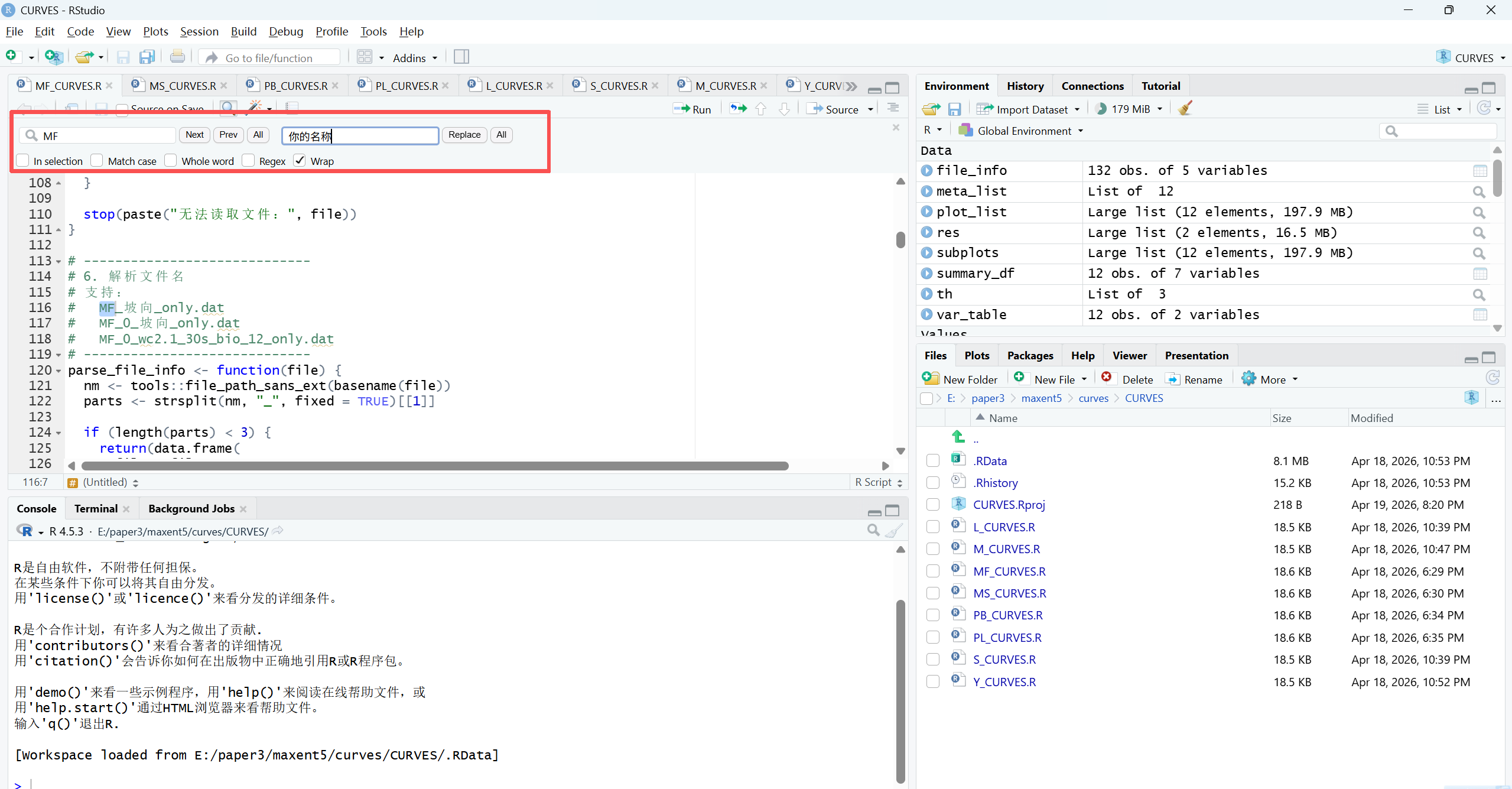
先修改好各种文件目录,然后在脚本区域按Ctrl+F,左边输入MF,右边输入你的物种名,点击ALL就可以将MF全部替换为你的物种名