第七章回归案例（二）美国爱荷华州埃姆斯地区房价预测

案例：美国爱荷华州埃姆斯地区房价预测

案例背景

本小节的案例的背景是对美国爱荷华州埃姆斯地区的房价进行预测。训练集中有共有1460条数据，81个特征，目标特征为该地区的房价。藉由此案例来简单说明正则化方法在实际案例中的运用

数据读取与划分

python 复制代码

## 载入所需要的模块和函数
import numpy as np
import pandas as pd
import matplotlib.pyplot as plt
import seaborn as sns
from scipy import stats
from scipy.stats import norm, skew

train = pd.read_csv('./input/train.csv')
## 查看所有特征的名称及数据类型
names = train.columns   ## 特征名称
types = train.dtypes    ## 数据类型

train.head()

| | Id | MSSubClass | MSZoning | LotFrontage | LotArea | Street | Alley | LotShape | LandContour | Utilities | ... | PoolArea | PoolQC | Fence | MiscFeature | MiscVal | MoSold | YrSold | SaleType | SaleCondition | SalePrice |
| 0 | 1 | 60 | RL | 65.0 | 8450 | Pave | NaN | Reg | Lvl | AllPub | ... | 0 | NaN | NaN | NaN | 0 | 2 | 2008 | WD | Normal | 208500 |
| 1 | 2 | 20 | RL | 80.0 | 9600 | Pave | NaN | Reg | Lvl | AllPub | ... | 0 | NaN | NaN | NaN | 0 | 5 | 2007 | WD | Normal | 181500 |
| 2 | 3 | 60 | RL | 68.0 | 11250 | Pave | NaN | IR1 | Lvl | AllPub | ... | 0 | NaN | NaN | NaN | 0 | 9 | 2008 | WD | Normal | 223500 |
| 3 | 4 | 70 | RL | 60.0 | 9550 | Pave | NaN | IR1 | Lvl | AllPub | ... | 0 | NaN | NaN | NaN | 0 | 2 | 2006 | WD | Abnorml | 140000 |

4	5	60	RL	84.0	14260	Pave	NaN	IR1	Lvl	AllPub	...	0	NaN	NaN	NaN	0	12	2008	WD	Normal	250000

5 rows × 81 columns

python 复制代码

## 删除无用特征"ID"
train.drop('Id', axis=1, inplace=True)

数据预处理：

异常点：

训练集中可能存在异常点，它们对模型的预测会产生不好的效果，所以我们要把它们从训练集中去掉。

python 复制代码

## 寻找异常点
fig, ax = plt.subplots()
ax.scatter(x = train['GrLivArea'], y = train['SalePrice'])
plt.ylabel('SalePrice', fontsize=13)
plt.xlabel('GrLivArea', fontsize=13)
plt.show()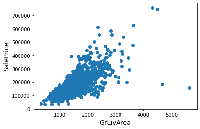

通过散点图可以发现，Saleprice应该随着GrLivArea的增大而增大，显然图的右下角的两个点为异常点，要将它们删除。

python 复制代码

## 删除异常点
train = train.drop(train[(train['GrLivArea']>4000) & (train['SalePrice']<300000)].index)

目标特征：SalePrice是我们需要去预测的，所以我们先要对这个特征进行一些分析。

python 复制代码

## 画出目标特征的密度直方图与核密度估计曲线，并画出正态曲线进行对比
sns.distplot(train['SalePrice'] , fit=norm)
plt.ylabel('Frequency')
plt.title('SalePrice distribution')

## QQ-图
fig = plt.figure()
res = stats.probplot(train['SalePrice'], plot=plt)
plt.show()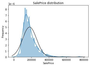

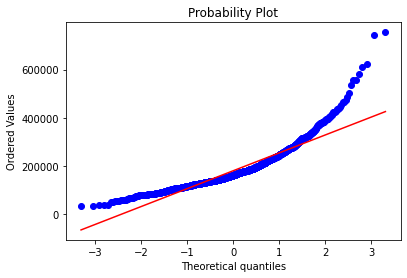
从上面两幅图可以看出SalePrice的分布不是正态分布，而且是右偏的。线性模型比较喜爱正态分布的数据，所以我们需要对这个特征进行变换，使其近似满足正态分布。

我们选择对目标特征进行对数变换：

python 复制代码

## 对数变换
train["SalePrice"] = np.log1p(train["SalePrice"])

## 再画出密度直方图和QQ-图观察效果
sns.distplot(train['SalePrice'] , fit=norm)
plt.ylabel('Frequency')
plt.title('SalePrice distribution')

fig = plt.figure()
res = stats.probplot(train['SalePrice'], plot=plt)
plt.show()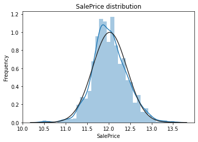

对数变换后的目标特征已经很接近于一个正态分布了。

缺失值处理：我们首先看看训练集中的缺失值统计：

python 复制代码

## 缺失值统计

# 计算缺失值的百分比
train_na = (train.isnull().sum() / len(train)) * 100
# 去掉没有缺失值的索引，其余的按降序排列
train_na = train_na.drop(train_na[train_na == 0].index).sort_values(ascending=False)   
# 生成数据框
missing_data = pd.DataFrame({'Missing Ratio' :train_na}) 
# 查看前10行
missing_data.head(10)

| | Missing Ratio |
| PoolQC | 99.588477 |
| MiscFeature | 96.296296 |
| Alley | 93.758573 |
| Fence | 80.727023 |
| FireplaceQu | 47.325103 |
| LotFrontage | 17.764060 |
| GarageType | 5.555556 |
| GarageYrBlt | 5.555556 |
| GarageFinish | 5.555556 |

GarageQual	5.555556

python 复制代码

## 缺失值条形图
f, ax = plt.subplots(figsize=(15, 12))
plt.xticks(rotation=90)
sns.barplot(x=train_na.index, y=train_na)
plt.xlabel('Features', fontsize=15)
plt.xticks(fontsize=15)
plt.ylabel('Percent of missing values', fontsize=15)
plt.xticks(fontsize=15)
plt.title('Percent missing data by feature', fontsize=15)
plt.show()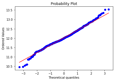

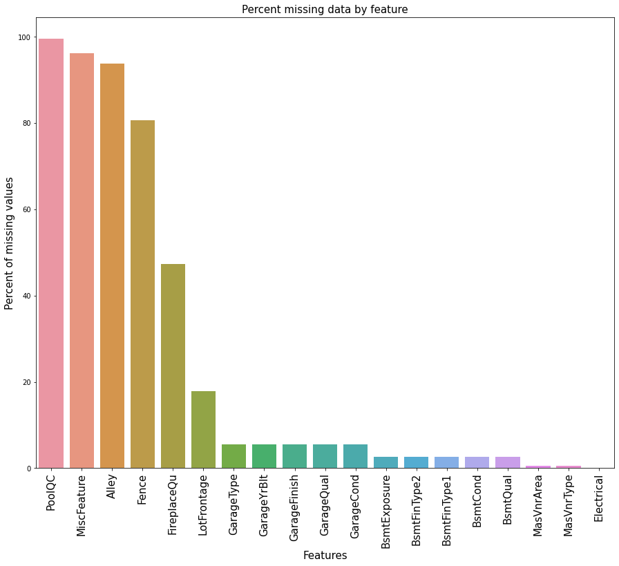
下面我们进行缺失值的插补：
PoolQC(泳池质量)：'NA'意味着没有泳池，所以其缺失率才会达到99%，我们用'None'来替代'NA'，对其它有此情况的特征也进行相应的插补。
GarageType(车库类型)， GarageFinish(车库内部装修)， GarageQual(车库质量)和GarageCond(车库条件)：用'None'来进行插补。
BsmtQual(地下室质量)，BsmtCond(地下室条件)，BsmtExposure(失修的地下室墙壁)，BsmtFinType1(地下室完成区域质量)和BsmtFinType2(地下室第二个区域完成质量)：我们用'None'对缺失值进行插补。
MasVnrType(砌体类型)用'None'来插补Type中的缺失值。
MSSubClass(建筑类)：用'None'进行插补

python 复制代码

fill_none_columns = ('PoolQC','MiscFeature','Alley','Fence','FireplaceQu','GarageType', 'GarageFinish', 'GarageQual', 'GarageCond','BsmtQual', 'BsmtCond', 'BsmtExposure', 'BsmtFinType1', 'BsmtFinType2',"MasVnrType","MSSubClass")
for col in fill_none_columns:
    train[col] = train[col].fillna('None')

接着集中将一些变量的缺失值填充为0
GarageYrBlt(车库修建年份)， GarageArea(车库面积)和GarageCars(车库容量),BsmtFinSF1(1型地下室面积)，BsmtFinSF2(2型地下室面积)，BsmtUnfSF(未完成的地下室面积)，TotalBsmtSF(地下室总面积),BsmtFullBath(全地下室浴室),BsmtHalfBath(半地下室浴室),MasVnrArea(砌体面积)对于这些变量我们使用0对其中的缺失值进行插补

python 复制代码

fill_zero_columns = ('GarageYrBlt', 'GarageArea', 'GarageCars','BsmtFinSF1', 'BsmtFinSF2', 'BsmtUnfSF','TotalBsmtSF', 'BsmtFullBath', 'BsmtHalfBath','MasVnrArea')
for col in fill_zero_columns:
    train[col] = train[col].fillna(0)

LotFrontage(连接到房产的街道的线性脚)：我们用邻近地区的LotFrontage的中位数来进行插补。

python 复制代码

train["LotFrontage"] = train.groupby("Neighborhood")["LotFrontage"].transform(
    lambda x: x.fillna(x.median()))

Functional(家庭功能评级)：数据集描述中表明'NA'意味着'typical'。

python 复制代码

train["Functional"] = train["Functional"].fillna("Typ")

Electrical(电力系统)和KitchenQual(厨房质量)：这两个变量只有一个缺失值，我们选择用众数进行插补。

python 复制代码

train['Electrical'] = train['Electrical'].fillna(train['Electrical'].mode()[0])
train['KitchenQual'] = train['KitchenQual'].fillna(train['KitchenQual'].mode()[0])

Exterior1st(房屋外墙),Exterior2nd(多于一种的房屋外墙),SaleType(销售类型)和MSZoning(地区分类)：直接用众数进行插补。

python 复制代码

train['Exterior1st'] = train['Exterior1st'].fillna(train['Exterior1st'].mode()[0])
train['Exterior2nd'] = train['Exterior2nd'].fillna(train['Exterior2nd'].mode()[0])
train['SaleType'] = train['SaleType'].fillna(train['SaleType'].mode()[0])
train['MSZoning'] = train['MSZoning'].fillna(train['MSZoning'].mode()[0])

Utilities(可用设备)：这个特征对模型预测没有帮助，我们可以放心删除它。

python 复制代码

train = train.drop(['Utilities'], axis=1)

最后我们再检查一下是否还存在缺失值：

python 复制代码

train_na = (train.isnull().sum() / len(train)) * 100
train_na = train_na.drop(train_na[train_na == 0].index).sort_values(ascending=False)
missing_data = pd.DataFrame({'Missing Ratio' :train_na})
missing_data.head()

	Missing Ratio

结果显示已经不存在缺失值了。

之后我们将部分数值特征转换为分类特征：

python 复制代码

train['MSSubClass'] = train['MSSubClass'].apply(str)
train['OverallCond'] = train['OverallCond'].astype(str)
train['YrSold'] = train['YrSold'].astype(str)
train['MoSold'] = train['MoSold'].astype(str)

进行分类特征的编码：

python 复制代码

from sklearn.preprocessing import LabelEncoder
cols = ('FireplaceQu', 'BsmtQual', 'BsmtCond', 'GarageQual', 'GarageCond', 
        'ExterQual', 'ExterCond','HeatingQC', 'PoolQC', 'KitchenQual', 'BsmtFinType1', 
        'BsmtFinType2', 'Functional', 'Fence', 'BsmtExposure', 'GarageFinish', 'LandSlope',
        'LotShape', 'PavedDrive', 'Street', 'Alley', 'CentralAir', 'MSSubClass', 'OverallCond', 
        'YrSold', 'MoSold')

for c in cols:
    lbl = LabelEncoder() 
    lbl.fit(list(train[c].values)) 
    train[c] = lbl.transform(list(train[c].values))

添加重要特征：因为与面积相关的特征对于房价的预测非常重要，所以我们又增加了每栋房子地下室，一层和二层的总面积这个特征。

python 复制代码

train['TotalSF'] = train['TotalBsmtSF'] + train['1stFlrSF'] + train['2ndFlrSF']

数值特征的偏度：

python 复制代码

numeric_feats = train.dtypes[train.dtypes != "object"].index

# 查看所有数值特征的偏度
skewed_feats = train[numeric_feats].apply(lambda x: skew(x.dropna())).sort_values(ascending=False)
skewness = pd.DataFrame({'Skew' :skewed_feats})
skewness.head(5)

| | Skew |
| MiscVal | 24.434913 |
| PoolArea | 15.932532 |
| LotArea | 12.560986 |
| 3SsnPorch | 10.286510 |

LowQualFinSF	8.995688

我们对偏度大于0.75的特征进行Box-Cox变换，使变换后的特征近似服从正态分布。

python 复制代码

from scipy.special import boxcox1p
skewness = skewness[abs(skewness) > 0.75]

skewed_features = skewness.index
lam = 0.15              # λ的取值为0.15
for feat in skewed_features:
    train[feat] = boxcox1p(train[feat], lam)

对分类特征进行哑编码：

python 复制代码

train = pd.get_dummies(train)
print(train.shape)

复制代码

(1458, 221)

模型搭建与训练

我们利用Python中的Sklearn模块进行建模。

python 复制代码

## 载入相应的模块和函数
from sklearn.linear_model import Lasso 
from sklearn.kernel_ridge import KernelRidge
from sklearn.pipeline import make_pipeline
from sklearn.preprocessing import RobustScaler
from sklearn.model_selection import KFold, cross_val_score
from sklearn.metrics import mean_squared_error

## 分离训练数据和标签
y_train = train.SalePrice
train.drop('SalePrice', axis=1, inplace=True)

我们还定义了交叉验证的策略，运用cross_val_score这个函数进行交叉验证，但其没有shuffle这个参数，于是我们又为此添加了一行代码，以便在交叉验证之前打乱训练集的顺序。

这里我们使用负均方误差作为评分标准

python 复制代码

n_folds = 5

def rmsle_cv(model):
    # 自己定义K折策略
    kf = KFold(n_folds, shuffle=True, random_state=42).get_n_splits(train.values)
    # 定义评价标准
    rmse= np.sqrt(-cross_val_score(model, train.values, y_train, scoring="neg_mean_squared_error", cv = kf))
    return(rmse)

基础模型：

Lasso：这个模型对异常点会比较敏感，所以在建模前先利用四分位数对数据进行缩放。

RobustScaler()：

根据四分位数来缩放数据，常常在数据有较多异常点的情况下使用。

python 复制代码

lasso = make_pipeline(RobustScaler(), Lasso(alpha =0.0005, random_state=1))

Kernel Ridge Regression：

python 复制代码

KRR = KernelRidge(alpha=0.6, kernel='polynomial', degree=2, coef0=2.5)

基础模型得分：

python 复制代码

score = []
model = [KRR, lasso]

for i in model:
    result = rmsle_cv(i)
    score.append(result.mean())

python 复制代码

model_name = ['Kernel Ridge Regression','Lasso']
result_score = pd.DataFrame({'model': model_name, 'score': score}, index=[1,2])
result_score

2	Lasso	0.014061

第七章 回归案例（二）美国爱荷华州埃姆斯地区房价预测

案例：美国爱荷华州埃姆斯地区房价预测

案例背景

数据读取与划分

模型搭建与训练

第七章回归案例（二）美国爱荷华州埃姆斯地区房价预测