Note：强化学习(四)

Note：强化学习(四)

2026 | ming

---

前面几章我们花了大量精力讨论 DQN 及其变体，本质上都是在做同一件事：努力学好一个动作价值函数 <math xmlns="http://www.w3.org/1998/Math/MathML"> Q ( s , a ) Q(s, a) </math>Q(s,a) ，然后让策略通过贪婪（或 <math xmlns="http://www.w3.org/1998/Math/MathML"> ϵ \epsilon </math>ϵ-贪婪）的方式 <math xmlns="http://www.w3.org/1998/Math/MathML"> a = arg ⁡ max ⁡ a Q ( s , a ) a = \arg\max_a Q(s, a) </math>a=argmaxaQ(s,a) 推导出来。这套基于价值的范式在 Atari 游戏上大杀四方，但如果你多训练几个环境就会皱眉头------它处理连续动作空间时效果并不理想。

这时候，就需要强化学习中的另一套体系登场了，它就是策略梯度法，那些知名的算法，比如PPO，A2C，TRPO，TD3等都是策略梯度法家族的成员。下面的这些章节我们就主要围绕策略梯度法展开。

策略梯度法与DQN之间的不同就是绕过 <math xmlns="http://www.w3.org/1998/Math/MathML"> Q Q </math>Q 函数这个中间商，直接去动策略的参数，让期望收益往上涨 。我们不再费劲地去评价某个动作"值多少钱"，而是直接参数化策略 <math xmlns="http://www.w3.org/1998/Math/MathML"> π θ ( a ∣ s ) \pi_\theta(a|s) </math>πθ(a∣s)，用神经网络输出动作的概率分布（离散）或高斯分布的均值方差（连续）。然后，我们顺着性能指标 <math xmlns="http://www.w3.org/1998/Math/MathML"> J ( θ ) J(\theta) </math>J(θ) 上升最快的方向 去调整参数 <math xmlns="http://www.w3.org/1998/Math/MathML"> θ \theta </math>θ。

十. REINFORCE 算法

10.1 数学原理

在强化学习的策略梯度算法家族中，REINFORCE 算法可以说是最基础、最直观的一员。它的核心思想很简单------直接对策略进行参数化，我们用神经网络模拟的不再是Q函数，而是策略函数 <math xmlns="http://www.w3.org/1998/Math/MathML"> π θ \pi_{\theta} </math>πθ，这个神经网络输入当前状态，输出每个动作的概率，因此只需通过最大化"策略带来的期望收益"来更新参数，无需像 Q 学习那样先学习价值函数再间接优化策略。

我们通常认为，智能体在环境中交互的过程，本质上就是采样一条"状态-动作-奖励"的时间序列，我们把这条序列称为轨迹 ，记为 <math xmlns="http://www.w3.org/1998/Math/MathML"> τ \tau </math>τ：
<math xmlns="http://www.w3.org/1998/Math/MathML" display="block"> τ = ( S 0 , A 0 , R 0 , S 1 , A 1 , R 1 , . . . , S T + 1 ) \tau = (S_{0},A_{0},R_{0},S_{1},A_{1},R_{1},...,S_{T+1}) </math>τ=(S0,A0,R0,S1,A1,R1,...,ST+1)

其中 <math xmlns="http://www.w3.org/1998/Math/MathML"> T T </math>T 是轨迹的终止时刻， <math xmlns="http://www.w3.org/1998/Math/MathML"> S T + 1 S_{T+1} </math>ST+1 通常是终止状态（无后续动作和奖励）。有了轨迹，我们就可以计算这条轨迹的总收益 （也叫累积奖励），需要注意的是，未来的奖励会有折扣因子 <math xmlns="http://www.w3.org/1998/Math/MathML"> γ \gamma </math>γ（ <math xmlns="http://www.w3.org/1998/Math/MathML"> 0 ≤ γ ≤ 1 0 \leq \gamma \leq 1 </math>0≤γ≤1），这符合我们的直观认知------近期的奖励比远期的奖励更有价值：
<math xmlns="http://www.w3.org/1998/Math/MathML" display="block"> G τ = R 0 + γ R 1 + γ 2 R 2 + . . . + γ T R T G_{\tau} = R_{0} + \gamma R_{1} + \gamma^{2}R_{2} + ... + \gamma^{T}R_{T} </math>Gτ=R0+γR1+γ2R2+...+γTRT

我们把策略参数化为 <math xmlns="http://www.w3.org/1998/Math/MathML"> π θ ( A ∣ S ) \pi_{\theta}(A|S) </math>πθ(A∣S)，表示在状态 <math xmlns="http://www.w3.org/1998/Math/MathML"> S S </math>S 下，参数为 <math xmlns="http://www.w3.org/1998/Math/MathML"> θ \theta </math>θ 的策略选择动作 <math xmlns="http://www.w3.org/1998/Math/MathML"> A A </math>A 的概率（实际实现中，我们用神经网络来建模这个策略，输出层用 softmax 激活得到每个动作的概率）。

REINFORCE 的目标很明确：找到最优的参数 <math xmlns="http://www.w3.org/1998/Math/MathML"> θ \theta </math>θ，使得策略 <math xmlns="http://www.w3.org/1998/Math/MathML"> π θ \pi_{\theta} </math>πθ 产生的期望收益 最大。因此，我们定义目标函数 <math xmlns="http://www.w3.org/1998/Math/MathML"> J ( θ ) J(\theta) </math>J(θ) 为轨迹收益的期望：
<math xmlns="http://www.w3.org/1998/Math/MathML" display="block"> J ( θ ) = E τ ∼ π θ [ G ( τ ) ] J(\theta) = E_{\tau \sim \pi_{\theta}}[G(\tau)] </math>J(θ)=Eτ∼πθ[G(τ)]

这里的期望可以直观理解为：多次用当前策略 <math xmlns="http://www.w3.org/1998/Math/MathML"> π θ \pi_{\theta} </math>πθ 采样轨迹，计算每条轨迹的收益 <math xmlns="http://www.w3.org/1998/Math/MathML"> G ( τ ) G(\tau) </math>G(τ)，再对所有收益取平均------这个平均值就是当前策略的"性能指标"，我们的目标就是通过调整 <math xmlns="http://www.w3.org/1998/Math/MathML"> θ \theta </math>θ，让这个指标尽可能大。

要最大化 <math xmlns="http://www.w3.org/1998/Math/MathML"> J ( θ ) J(\theta) </math>J(θ)，我们采用梯度上升法（因为是最大化目标，而非最小化损失），核心是求出 <math xmlns="http://www.w3.org/1998/Math/MathML"> ∇ θ J ( θ ) \nabla_{\theta}J(\theta) </math>∇θJ(θ)，也就是目标函数对参数 <math xmlns="http://www.w3.org/1998/Math/MathML"> θ \theta </math>θ 的梯度。

由于期望的梯度难以直接计算，我们通常采用蒙特卡洛采样 的方式来近似：先采样 <math xmlns="http://www.w3.org/1998/Math/MathML"> n n </math>n 条轨迹 <math xmlns="http://www.w3.org/1998/Math/MathML"> τ ( 1 ) , τ ( 2 ) , . . . , τ ( n ) \tau^{(1)}, \tau^{(2)}, ..., \tau^{(n)} </math>τ(1),τ(2),...,τ(n)（每条轨迹都服从当前策略 <math xmlns="http://www.w3.org/1998/Math/MathML"> π θ \pi_{\theta} </math>πθ），再用这些轨迹的收益来近似梯度。

首先，单条轨迹 <math xmlns="http://www.w3.org/1998/Math/MathML"> τ ( i ) \tau^{(i)} </math>τ(i) 对梯度的贡献可以表示为（如下公式的数学推导比较繁琐复杂，没有一定数学基础的同学可能看不懂其推导过程，所以这里就没有解释这个公式是怎么来的，不过，相信凭借你的直觉，也能看懂这个公式到底在做什么）：
<math xmlns="http://www.w3.org/1998/Math/MathML" display="block"> x ( i ) = ∇ θ ∑ t = 0 T G ( τ ( i ) ) l o g π θ ( A t ( i ) ∣ S t ( i ) ) x^{(i)}=\nabla_{\theta}\sum_{t=0}^{T}G(\tau^{(i)})log \space \pi_{\theta}(A_{t}^{(i)}|S_{t}^{(i)}) </math>x(i)=∇θt=0∑TG(τ(i))log πθ(At(i)∣St(i))

然后，整个目标函数的梯度就是所有采样轨迹贡献的平均值：
<math xmlns="http://www.w3.org/1998/Math/MathML" display="block"> ∇ θ J ( θ ) = x ( 1 ) + x ( 2 ) + ⋯ + x ( n ) n \nabla_{\theta}J(\theta) =\frac{x^{(1)}+x^{(2)}+\cdots +x^{(n)}}{n} </math>∇θJ(θ)=nx(1)+x(2)+⋯+x(n)

这里直观解读一下这个梯度公式： <math xmlns="http://www.w3.org/1998/Math/MathML"> l o g π θ ( A t ∣ S t ) log \space \pi_{\theta}(A_t|S_t) </math>log πθ(At∣St) 表示"在状态 <math xmlns="http://www.w3.org/1998/Math/MathML"> S t S_t </math>St 下选择动作 <math xmlns="http://www.w3.org/1998/Math/MathML"> A t A_t </math>At 的对数概率"，其梯度反映了"调整参数 <math xmlns="http://www.w3.org/1998/Math/MathML"> θ \theta </math>θ 能多大程度改变这个动作的选择概率"；而 <math xmlns="http://www.w3.org/1998/Math/MathML"> G ( τ ) G(\tau) </math>G(τ) 作为权重，相当于在告诉算法------如果这条轨迹的总收益高，我们就希望增大这条轨迹中所有动作的选择概率；如果收益低，我们就希望减小这些动作的选择概率。

但是，上面的公式有一个明显的问题：我们用整条轨迹的总收益 <math xmlns="http://www.w3.org/1998/Math/MathML"> G ( τ ) G(\tau) </math>G(τ) 作为所有时刻动作的权重，但实际上，一个动作的好坏，只应该由它之后的奖励来决定------动作发生之前的奖励，和这个动作的价值毫无关系。

举个例子：假设一条轨迹的前半段运气好拿到了高奖励，后半段动作很差但总收益依然不低，此时用总收益作为权重，会错误地增大后半段差动作的选择概率，这会引入不必要的噪声，影响算法收敛。

为了解决这个问题，我们将总收益 <math xmlns="http://www.w3.org/1998/Math/MathML"> G ( τ ) G(\tau) </math>G(τ) 替换为时序差分收益 <math xmlns="http://www.w3.org/1998/Math/MathML"> G t ( τ ) G_t(\tau) </math>Gt(τ)，即时刻 <math xmlns="http://www.w3.org/1998/Math/MathML"> t t </math>t 之后的累积奖励：
<math xmlns="http://www.w3.org/1998/Math/MathML" display="block"> G t ( τ ) = R t + γ R t + 1 + . . . + γ T − t R T G_{t}(\tau) = R_{t} + \gamma R_{t+1} + ... + \gamma^{T-t}R_{T} </math>Gt(τ)=Rt+γRt+1+...+γT−tRT

此时，梯度公式就修正为：
<math xmlns="http://www.w3.org/1998/Math/MathML" display="block"> x ( i ) = ∇ θ ∑ t = 0 T G t ( τ ( i ) ) l o g π θ ( A t ( i ) ∣ S t ( i ) ) x^{(i)}=\nabla_{\theta}\sum_{t=0}^{T}G_{t}(\tau^{(i)})log \space \pi_{\theta}(A_{t}^{(i)}|S_{t}^{(i)}) </math>x(i)=∇θt=0∑TGt(τ(i))log πθ(At(i)∣St(i))

这个修正看似简单，却能极大地降低梯度估计的方差------因为每个动作的权重只和它之后的奖励相关，排除了之前无关奖励的干扰，这也是 REINFORCE 算法能稳定收敛的关键改进。

10.2 代码实现

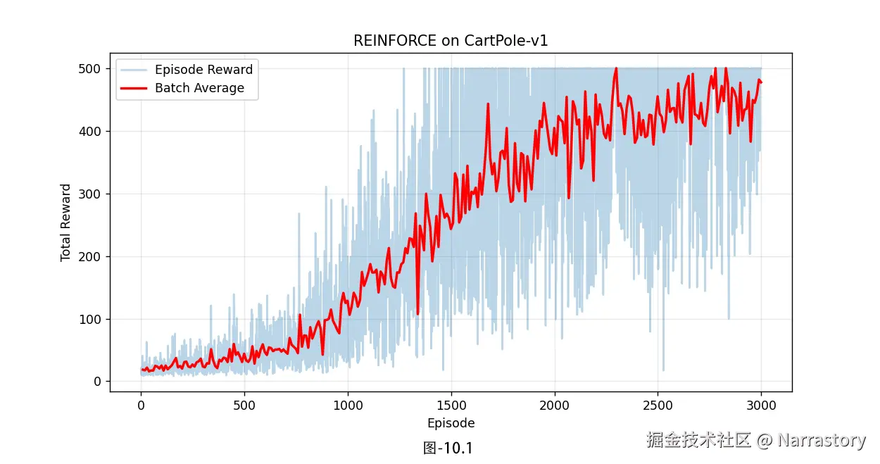
如下是一个标准的REINFORCE 算法代码实现，并且在gymnasium库的CartPole-v1离散环境上进行测试，效果还是很不错的。这个代码非常易读，如果你要在其它环境使用REINFORCE 算法，那么只需要稍微修改一下此代码即可。

import torch
import torch.nn as nn
import torch.optim as optim
import gymnasium as gym
import matplotlib.pyplot as plt
from tqdm import tqdm
from typing import List, Tuple


# ==================== 策略网络 ====================
class PolicyNet(nn.Module):
    """简单的两层全连接网络，输出动作概率分布"""
    def __init__(self, state_dim: int, action_dim: int, hidden_dim: int = 128):
        super().__init__()
        self.net = nn.Sequential(
            nn.Linear(state_dim, hidden_dim),
            nn.ReLU(),
            nn.Linear(hidden_dim, action_dim),
            nn.Softmax(dim=-1)          # 确保输出是合法的概率分布
        )

    def forward(self, x: torch.Tensor) -> torch.Tensor:
        return self.net(x)


# ==================== REINFORCE Agent ====================
class REINFORCEAgent:
    """
    蒙特卡洛策略梯度（REINFORCE）算法的实现。
    核心思想：用整条轨迹的累积回报 G_t 作为权重，增加"好动作"的概率，
             减少"坏动作"的概率。
    """
    def __init__(
        self,
        state_dim: int,
        action_dim: int,
        lr: float = 1e-3,
        gamma: float = 0.99,
        trajectories_per_update: int = 10
    ):
        self.gamma = gamma
        self.trajectories_per_update = trajectories_per_update

        self.policy_net = PolicyNet(state_dim, action_dim)
        self.optimizer = optim.Adam(self.policy_net.parameters(), lr=lr)

        # 存储当前 batch 的所有轨迹数据
        # 每条轨迹是一个三元组列表：[(state, action, reward), ...]
        self.trajectories: List[List[Tuple[torch.Tensor, int, float]]] = []

    def get_action(self, state: torch.Tensor) -> Tuple[int, torch.Tensor]:
        """
        根据当前策略采样一个动作。
        返回：
            action (int): 执行的动作编号
            log_prob (torch.Tensor): 该动作的对数概率，用于后续梯度计算
        """
        state = state.unsqueeze(0)                     # [1, state_dim]
        probs = self.policy_net(state).squeeze(0)      # [action_dim]
        dist = torch.distributions.Categorical(probs)
        action = dist.sample()
        log_prob = dist.log_prob(action)               # 直接获取 log π(a|s)

        return action.item(), log_prob

    def store_trajectory(self, trajectory: List[Tuple[torch.Tensor, int, float]]):
        """存储一条完整的轨迹，等到 batch 足够时再更新"""
        self.trajectories.append(trajectory)

    def update(self) -> float:
        """
        使用当前 batch 内的所有轨迹执行一次策略梯度更新。
        返回本次更新的平均损失值，便于监控训练进程。
        """
        if len(self.trajectories) < self.trajectories_per_update:
            return 0.0

        batch_loss = []
        self.optimizer.zero_grad()

        for trajectory in self.trajectories:
            # 1. 计算每个时间步的累积回报 G_t（从后向前递推）
            returns = []
            G = 0.0
            for _, _, reward in reversed(trajectory):
                G = reward + self.gamma * G
                returns.insert(0, G)            # 保持时间步顺序

            returns = torch.tensor(returns, dtype=torch.float32)

            # 2. 收集这条轨迹的所有对数概率
            log_probs = torch.stack([step[1] for step in trajectory])

            # 3. 策略梯度损失：L = - Σ log π(a_t|s_t) * G_t
            #    取负号是因为优化器做的是梯度下降，而策略梯度本质是梯度上升
            trajectory_loss = - (log_probs * returns).sum()
            batch_loss.append(trajectory_loss)

        # 对 batch 内所有轨迹的损失求平均，然后反向传播
        total_loss = torch.stack(batch_loss).mean()
        total_loss.backward()
        self.optimizer.step()

        # 清空已使用的轨迹，准备收集下一批
        self.trajectories.clear()

        return total_loss.item()


# ==================== 训练循环 ====================
def train_reinforce(
    env_name: str = "CartPole-v1",
    num_episodes: int = 500,
    trajectories_per_update: int = 10,
    gamma: float = 0.99,
    lr: float = 1e-3,
    seed: int = 42
):
    """REINFORCE 训练主函数"""
    torch.manual_seed(seed)
    env = gym.make(env_name)
    state_dim = env.observation_space.shape[0]
    action_dim = env.action_space.n

    agent = REINFORCEAgent(
        state_dim=state_dim,
        action_dim=action_dim,
        lr=lr,
        gamma=gamma,
        trajectories_per_update=trajectories_per_update
    )

    episode_rewards = []          # 记录每个 episode 的总奖励
    avg_rewards = []              # 记录滑动平均奖励（用于绘图）

    pbar = tqdm(range(num_episodes), desc="Training REINFORCE")
    for episode in pbar:
        state, _ = env.reset()
        done = False
        episode_reward = 0.0
        trajectory = []           # 存储当前 episode 的 (state, log_prob, reward)

        while not done:
            state_tensor = torch.tensor(state, dtype=torch.float32)
            action, log_prob = agent.get_action(state_tensor)

            next_state, reward, terminated, truncated, _ = env.step(action)
            done = terminated or truncated

            # 存储这一步的信息（状态、对数概率、奖励）
            trajectory.append((state_tensor, log_prob, reward))

            state = next_state
            episode_reward += reward

        # 一条完整轨迹结束，存起来
        agent.store_trajectory(trajectory)
        episode_rewards.append(episode_reward)

        # 当收集够指定数量的轨迹时，执行一次策略更新
        if (episode + 1) % trajectories_per_update == 0:
            loss = agent.update()
            avg_reward = sum(episode_rewards[-trajectories_per_update:]) / trajectories_per_update
            avg_rewards.append(avg_reward)
            pbar.set_postfix({
                "Avg Reward": f"{avg_reward:.2f}",
                "Loss": f"{loss:.4f}" if loss else "N/A"
            })

    env.close()
    return avg_rewards, episode_rewards


# ==================== 运行与绘图 ====================
if __name__ == "__main__":
    avg_rewards, all_rewards = train_reinforce(
        num_episodes=3000,
        trajectories_per_update=10,
        gamma=0.99,
        lr=1e-3
    )

    plt.figure(figsize=(10, 5))
    plt.plot(all_rewards, alpha=0.3, label="Episode Reward")
    # 绘制每 batch 的平均奖励
    batch_indices = range(9, len(all_rewards), 10)   # 10 条轨迹一个 batch
    plt.plot(batch_indices, avg_rewards, 'r-', linewidth=2, label="Batch Average")
    plt.xlabel("Episode")
    plt.ylabel("Total Reward")
    plt.title("REINFORCE on CartPole-v1")
    plt.legend()
    plt.grid(True, alpha=0.3)
    plt.show()

输出结果图10.1：

十一. Actor-Critic 算法

11.1 数学原理

在我们熟悉的强化学习算法中，策略梯度（比如 REINFORCE）和价值函数方法（比如 DQN）各有优劣------策略梯度能直接优化策略，但方差大、样本效率低；价值函数能提供更稳定的信号，却只能间接地指导策略更新。而 Actor-Critic（AC）算法，本质上就是把这两者结合起来，让它们"分工协作"，既解决策略梯度的方差问题，又提升训练的稳定性和效率，这也是它成为现代强化学习核心算法之一的原因。

我们先回顾一下基础的策略梯度公式，这是理解 AC 算法的起点。原始的策略梯度目标函数梯度为：
<math xmlns="http://www.w3.org/1998/Math/MathML" display="block"> ∇ θ J ( θ ) = E τ ∼ π θ [ ∇ θ ∑ t = 0 T G t ( τ ) log ⁡ π θ ( A t ∣ S t ) ] \nabla_{\theta}J(\theta) = E_{\tau \sim \pi_{\theta}}[\nabla_{\theta}\sum_{t=0}^{T}G_{t}(\tau)\log \space \pi_{\theta}(A_{t}|S_{t})] </math>∇θJ(θ)=Eτ∼πθ[∇θt=0∑TGt(τ)log πθ(At∣St)]

这里的 <math xmlns="http://www.w3.org/1998/Math/MathML"> G t ( τ ) G_{t}(\tau) </math>Gt(τ)是轨迹 <math xmlns="http://www.w3.org/1998/Math/MathML"> τ \tau </math>τ在时刻 t 的累积回报，也就是我们常说的"未来总收益"。但实际训练中我们会发现， <math xmlns="http://www.w3.org/1998/Math/MathML"> G t ( τ ) G_{t}(\tau) </math>Gt(τ)的波动非常大------同样的状态动作对，在不同轨迹中可能得到完全不同的累积回报，这就导致策略梯度的方差极大。

方差大带来的问题很直观：训练过程不稳定，需要大量样本才能收敛，甚至可能出现训练无效的情况（比如某个状态本身就是"死局"，无论采取什么动作，未来回报都极低，此时基于 <math xmlns="http://www.w3.org/1998/Math/MathML"> G t ( τ ) G_{t}(\tau) </math>Gt(τ)的更新就是无用功）。

解决这个问题的核心思路很简单：给波动的 <math xmlns="http://www.w3.org/1998/Math/MathML"> G t ( τ ) G_{t}(\tau) </math>Gt(τ)"去噪"------减去一个固定的均值，让梯度的波动范围缩小，从而提升样本效率。而这个"均值"，我们通常会用价值函数来替代，这就是 AC 算法的核心灵感。

当我们用价值函数 <math xmlns="http://www.w3.org/1998/Math/MathML"> V ω ( S t ) V_{\omega}(S_{t}) </math>Vω(St)（其中 <math xmlns="http://www.w3.org/1998/Math/MathML"> ω \omega </math>ω是价值函数模型的参数）作为"均值"时，策略梯度公式就被修改为：
<math xmlns="http://www.w3.org/1998/Math/MathML" display="block"> ∇ θ J ( θ ) = E τ ∼ π θ [ ∇ θ ∑ t = 0 T ( G t ( τ ) − V ω ( S t ) ) log ⁡ π θ ( A t ∣ S t ) ] \nabla_{\theta}J(\theta) = E_{\tau \sim \pi_{\theta}}[\nabla_{\theta}\sum_{t=0}^{T}(G_{t}(\tau) - V_{\omega}(S_{t}))\log \space \pi_{\theta}(A_{t}|S_{t})] </math>∇θJ(θ)=Eτ∼πθ[∇θt=0∑T(Gt(τ)−Vω(St))log πθ(At∣St)]

这里的 <math xmlns="http://www.w3.org/1998/Math/MathML"> G t ( τ ) − V ω ( S t ) G_{t}(\tau) - V_{\omega}(S_{t}) </math>Gt(τ)−Vω(St)，其实就是我们常说的"优势"------它衡量了"实际累积回报"比"当前状态的预期价值"高多少（为正表示这个动作比预期好，为负则表示比预期差）。用优势替代原始的 <math xmlns="http://www.w3.org/1998/Math/MathML"> G t ( τ ) G_{t}(\tau) </math>Gt(τ)，相当于过滤了状态本身的固有价值，只关注动作带来的"额外收益"，方差自然就降低了。

到这里，我们其实已经有了 AC 算法的两个核心组件：

• Actor（演员） ：就是我们的策略模型 <math xmlns="http://www.w3.org/1998/Math/MathML"> π θ ( A t ∣ S t ) \pi_{\theta}(A_{t}|S_{t}) </math>πθ(At∣St)，负责根据当前状态输出动作，核心任务是通过梯度更新，最大化策略目标函数（也就是跟着"优势信号"走，多做能带来正优势的动作）。
• Critic（评论家） ：就是我们的价值函数模型 <math xmlns="http://www.w3.org/1998/Math/MathML"> V ω ( S t ) V_{\omega}(S_{t}) </math>Vω(St)，负责评估当前状态的价值，核心任务是准确预测 <math xmlns="http://www.w3.org/1998/Math/MathML"> V ω ( S t ) V_{\omega}(S_{t}) </math>Vω(St)，为 Actor 提供可靠的"均值"和优势信号。

上面的改进还有一个小问题：如果我们沿用蒙特卡洛方法来计算 <math xmlns="http://www.w3.org/1998/Math/MathML"> G t ( τ ) G_{t}(\tau) </math>Gt(τ)，就必须等到整个轨迹结束（抵达目标或终止状态），才能得到 <math xmlns="http://www.w3.org/1998/Math/MathML"> G t ( τ ) G_{t}(\tau) </math>Gt(τ)的值，进而更新 Actor 和 Critic 的参数。这显然不够高效------很多时候，我们希望算法能"边探索边更新"，不用等到轨迹结束就能调整参数。

解决这个问题的关键，就是引入 TD（时序差分）方法。我们知道，TD 方法的核心是用"即时奖励 + 下一状态的预期价值"来近似当前的累积回报，也就是：
<math xmlns="http://www.w3.org/1998/Math/MathML" display="block"> G t ( τ ) ≈ R t + γ V ω ( S t + 1 ) G_{t}(\tau) \approx R_{t} + \gamma V_{\omega}(S_{t+1}) </math>Gt(τ)≈Rt+γVω(St+1)

把这个近似代入策略梯度公式，就得到了 AC 算法中最常用的梯度更新形式：
<math xmlns="http://www.w3.org/1998/Math/MathML" display="block"> ∇ θ J ( θ ) = E τ ∼ π θ [ ∇ θ ∑ t = 0 T ( R t + γ V ω ( S t + 1 ) − V ω ( S t ) ) log ⁡ π θ ( A t ∣ S t ) ] \nabla_{\theta}J(\theta) = E_{\tau \sim \pi_{\theta}}[\nabla_{\theta}\sum_{t=0}^{T}(R_{t} + \gamma V_{\omega}(S_{t+1}) - V_{\omega}(S_{t}))\log \space \pi_{\theta}(A_{t}|S_{t})] </math>∇θJ(θ)=Eτ∼πθ[∇θt=0∑T(Rt+γVω(St+1)−Vω(St))log πθ(At∣St)]

这里有个很直观的点： <math xmlns="http://www.w3.org/1998/Math/MathML"> R t + γ V ω ( S t + 1 ) R_{t} + \gamma V_{\omega}(S_{t+1}) </math>Rt+γVω(St+1)其实就是对动作价值函数 <math xmlns="http://www.w3.org/1998/Math/MathML"> Q ( S t , A t ) Q(S_{t},A_{t}) </math>Q(St,At)的近似------它表示"当前动作带来的即时奖励 + 下一状态的预期价值"，刚好对应动作 <math xmlns="http://www.w3.org/1998/Math/MathML"> A t A_t </math>At 在当前状态 <math xmlns="http://www.w3.org/1998/Math/MathML"> S t S_t </math>St 下的价值。

所以，括号里的部分 <math xmlns="http://www.w3.org/1998/Math/MathML"> R t + γ V ω ( S t + 1 ) − V ω ( S t ) R_{t} + \gamma V_{\omega}(S_{t+1}) - V_{\omega}(S_{t}) </math>Rt+γVω(St+1)−Vω(St)，本质上就是优势函数 <math xmlns="http://www.w3.org/1998/Math/MathML"> A ( S t , A t ) = Q ( S t , A t ) − V ( S t ) A(S_{t},A_{t}) = Q(S_{t},A_{t}) - V(S_{t}) </math>A(St,At)=Q(St,At)−V(St)的近似。这一步改进后，我们就可以在轨迹推进的过程中，每一步都计算优势、更新 Actor 和 Critic 的参数，实现"在线更新"------不用等到轨迹结束，边走向目标边调整，训练速度和稳定性都得到了显著提升。

和单纯的策略梯度相比，AC 用价值函数降低了梯度方差，提升了样本效率；和单纯的价值函数方法相比，AC 能直接优化策略，避免了"价值函数最优但策略不最优"的问题。这也是为什么 AC 算法及其变体（比如 DDPG、PPO 中的 AC 结构），在复杂的强化学习任务中（比如连续动作空间）应用得如此广泛。

最后补充一句：实际实现中，Actor 和 Critic 通常都是用神经网络来建模。

11.2 代码实现

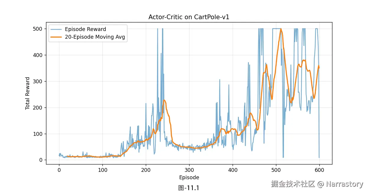
如下是一个简单但标准的ActorCritic算法代码实现，并且在gymnasium库的CartPole-v1离散环境上进行测试，效果还是很不错的。这个代码非常易读，如果你要在其它环境使用此算法，那么只需要稍微修改一下此代码即可。

import torch
import torch.nn as nn
import gymnasium as gym
import matplotlib.pyplot as plt
from tqdm import tqdm


# -------------------- 神经网络定义 --------------------
class PolicyNet(nn.Module):
    """策略网络：输出动作概率分布 π(a|s)"""

    def __init__(self, state_dim, action_dim):
        super().__init__()
        self.net = nn.Sequential(
            nn.Linear(state_dim, 128),
            nn.ReLU(),
            nn.Linear(128, 64),
            nn.ReLU(),
            nn.Linear(64, action_dim),
            nn.Softmax(dim=-1),  # 输出动作概率，和为 1
        )

    def forward(self, x):
        return self.net(x)


class ValueNet(nn.Module):
    """价值网络：估计状态价值 V(s)"""

    def __init__(self, state_dim):
        super().__init__()
        self.net = nn.Sequential(
            nn.Linear(state_dim, 128),
            nn.ReLU(),
            nn.Linear(128, 64),
            nn.ReLU(),
            nn.Linear(64, 1),  # 输出一个标量值
        )

    def forward(self, x):
        return self.net(x)


# -------------------- Actor-Critic 智能体 --------------------
class ActorCriticAgent:
    """
    Actor-Critic 智能体，采用单步 TD 误差更新：
        - Critic（价值网络）最小化 TD 误差的 MSE
        - Actor（策略网络）沿着 TD 误差乘以 log π 的梯度方向更新
    """

    def __init__(
        self, state_dim, action_dim, gamma=0.99, lr_policy=1e-3, lr_value=1e-3
    ):
        self.gamma = gamma  # 折扣因子
        self.state_dim = state_dim
        self.action_dim = action_dim

        # 初始化网络
        self.policy_net = PolicyNet(state_dim, action_dim)
        self.value_net = ValueNet(state_dim)

        # 优化器（可分别调节学习率）
        self.optimizer_policy = torch.optim.Adam(
            self.policy_net.parameters(), lr=lr_policy
        )
        self.optimizer_value = torch.optim.Adam(
            self.value_net.parameters(), lr=lr_value
        )

        # 损失函数
        self.mse_loss = nn.MSELoss()

        # 训练模式
        self.policy_net.train()
        self.value_net.train()

    def select_action(self, state):
        """
        根据当前策略采样一个动作。
        参数:
            state: Tensor, shape [state_dim]
        返回:
            action: int, 选择的动作编号
            log_prob: Tensor, 该动作对应的对数概率（用于后续策略梯度计算）
        """
        state = state.unsqueeze(0)  # 增加 batch 维度: [1, state_dim]
        probs = self.policy_net(state).squeeze(0)  # [action_dim]

        # 按概率分布采样动作
        action = torch.multinomial(probs, 1).item()

        # 计算该动作的对数概率
        log_prob = torch.log(probs[action] + 1e-8)  # 加上极小值防止 log(0)

        return action, log_prob

    def update(self, state, action_log_prob, reward, next_state, done):
        """
        执行一步 Actor-Critic 更新。
        参数:
            state:       当前状态 Tensor [state_dim]
            action_log_prob: 所执行动作的对数概率（标量 Tensor）
            reward:      即时奖励 (float)
            next_state:  下一状态 Tensor [state_dim]
            done:        是否终止 (bool)
        """
        # 添加 batch 维度: [1, state_dim]
        state = state.unsqueeze(0)
        next_state = next_state.unsqueeze(0)

        # ---- 1. 计算 TD 目标 ----
        with torch.no_grad():
            next_value = self.value_net(next_state) * (0.0 if done else 1.0)
            td_target = reward + self.gamma * next_value

        # 当前状态的价值估计
        value = self.value_net(state)

        # Critic 损失 (MSE)
        value_loss = self.mse_loss(value, td_target)

        # ---- 2. 计算 TD 误差（优势函数的近似） ----
        td_error = (td_target - value).detach()  # 阻断梯度，只作为 Actor 的权重

        # Actor 损失 (策略梯度，最大化期望回报等价于最小化 -logπ * δ)
        policy_loss = -action_log_prob * td_error

        # ---- 3. 梯度更新 ----
        self.optimizer_policy.zero_grad()
        self.optimizer_value.zero_grad()

        policy_loss.backward()
        value_loss.backward()

        self.optimizer_policy.step()
        self.optimizer_value.step()


# -------------------- 训练主循环 --------------------
def train_cartpole():
    # 环境配置
    env = gym.make("CartPole-v1")  # 经典平衡杆任务
    state_dim = env.observation_space.shape[0]  # 4
    action_dim = env.action_space.n  # 2

    agent = ActorCriticAgent(
        state_dim, action_dim, gamma=0.99, lr_policy=3e-4, lr_value=5e-4
    )

    num_episodes = 600	
    reward_history = []

    pbar = tqdm(range(num_episodes), desc="Training", ncols=100)
    for episode in pbar:
        state, _ = env.reset()
        state = torch.tensor(state, dtype=torch.float32)
        total_reward = 0.0
        done = False

        while not done:
            # 1. 选择动作
            action, log_prob = agent.select_action(state)

            # 2. 执行动作
            next_state, reward, terminated, truncated, _ = env.step(action)
            done = terminated or truncated
            next_state = torch.tensor(next_state, dtype=torch.float32)

            # 3. 智能体学习（在线更新）
            agent.update(state, log_prob, reward, next_state, done)

            # 4. 状态转移
            state = next_state
            total_reward += reward

        reward_history.append(total_reward)

        # 动态显示最近 10 局平均奖励
        if len(reward_history) >= 10:
            avg_reward = sum(reward_history[-10:]) / 10
            pbar.set_postfix({"avg_reward": f"{avg_reward:.2f}"})

    env.close()
    return reward_history


# -------------------- 可视化结果 --------------------
if __name__ == "__main__":
    rewards = train_cartpole()

    plt.figure(figsize=(10, 5))
    plt.plot(rewards, alpha=0.6, label="Episode Reward")
    # 绘制平滑曲线（滑动平均）
    window = 20
    smoothed = [
        sum(rewards[i : i + window]) / window for i in range(len(rewards) - window + 1)
    ]
    plt.plot(
        range(window - 1, len(rewards)),
        smoothed,
        linewidth=2,
        label=f"{window}-Episode Moving Avg",
    )
    plt.xlabel("Episode")
    plt.ylabel("Total Reward")
    plt.title("Actor-Critic on CartPole-v1")
    plt.legend()
    plt.grid(True, alpha=0.3)
    plt.show()

运行结果如图11.1所示，从图中可以清晰观察到，奖励（reward）曲线呈现出明显的动荡特征：前期快速攀升至500左右的峰值后，随即骤降至50附近，之后又逐步回升，后续仍有反复波动，整体稳定性欠佳。其实这就是 AC 算法的典型训练特性------训练过程易波动、收敛速度偏慢，核心原因在于 Actor 与 Critic 两个网络存在"互相影响、互相更新"的耦合关系：Critic 的价值评估精度直接决定了 Actor 梯度更新的可靠性，而 Actor 策略的变化又会导致环境交互数据分布改变，进而影响 Critic 的训练效果，这种双向耦合很容易引发训练震荡。

但即便存在这样的训练波动，AC 算法的潜力依然非常巨大，后面我们会针对这些痛点进行优化。

---

END~