DenseNet121学习笔记

🍨 本文为🔗365天深度学习训练营中的学习记录博客
🍖 原作者：K同学啊

一、前期准备

python 复制代码

import torch
import torch.nn as nn
import torch.nn.functional as F
from torchsummary import summary

二、定义核心组件：Dense Layer

python 复制代码

class DenseLayer(nn.Module):
    def __init__(self, num_input_features, growth_rate, bn_size, drop_rate):
        super(DenseLayer, self).__init__()
        # 1x1 卷积
        self.norm1 = nn.BatchNorm2d(num_input_features)
        self.relu1 = nn.ReLU(inplace=True)
        self.conv1 = nn.Conv2d(num_input_features, bn_size * growth_rate, kernel_size=1, stride=1, bias=False)
        
        # 3x3 卷积
        self.norm2 = nn.BatchNorm2d(bn_size * growth_rate)
        self.relu2 = nn.ReLU(inplace=True)
        self.conv2 = nn.Conv2d(bn_size * growth_rate, growth_rate, kernel_size=3, stride=1, padding=1, bias=False)
        
        self.drop_rate = drop_rate

    def forward(self, x):

        out = self.conv1(self.relu1(self.norm1(x)))
        out = self.conv2(self.relu2(self.norm2(out)))
        
        if self.drop_rate > 0:
            out = F.dropout(out, p=self.drop_rate, training=self.training)
        return out

三、组装：Dense Block

python 复制代码

class DenseBlock(nn.ModuleDict):
    def __init__(self, num_layers, num_input_features, bn_size, growth_rate, drop_rate):
        super(DenseBlock, self).__init__()
        for i in range(num_layers):
            layer = DenseLayer(
                num_input_features + i * growth_rate,
                growth_rate=growth_rate,
                bn_size=bn_size,
                drop_rate=drop_rate
            )
            self.add_module('denselayer%d' % (i + 1), layer)

    def forward(self, init_features):
        features = [init_features] # 这里依然是个列表
        for name, layer in self.items():
            # 在送入 layer 之前，先把它拼接成一个大 Tensor
            concated_features = torch.cat(features, 1) 
            
            # 把拼接好的 Tensor 送给 layer，这样 torchsummary 就不会懵了
            new_features = layer(concated_features) 
            features.append(new_features)
            
        return torch.cat(features, 1)

四、过渡组件：Transition Layer（过渡层）

python 复制代码

# 用于连接 Dense Block，降低通道数和特征图大小
class Transition(nn.Sequential):
    def __init__(self, num_input_features, num_output_features):
        super(Transition, self).__init__()
        self.add_module('norm', nn.BatchNorm2d(num_input_features))
        self.add_module('relu', nn.ReLU(inplace=True))
        # 1x1 卷积降低通道数
        self.add_module('conv', nn.Conv2d(num_input_features, num_output_features, kernel_size=1, stride=1, bias=False))
        # 2x2 平均池化缩小特征图尺寸
        self.add_module('pool', nn.AvgPool2d(kernel_size=2, stride=2))

五、构建完整的 DenseNet 网络

python 复制代码

class DenseNet(nn.Module):
    def __init__(self, growth_rate=32, block_config=(6, 12, 24, 16), num_init_features=64, bn_size=4, drop_rate=0, num_classes=1000):
        super(DenseNet, self).__init__()

        # 第一部分：最初的卷积层
        self.features = nn.Sequential(
            nn.Conv2d(3, num_init_features, kernel_size=7, stride=2, padding=3, bias=False),
            nn.BatchNorm2d(num_init_features),
            nn.ReLU(inplace=True),
            nn.MaxPool2d(kernel_size=3, stride=2, padding=1)
        )

        # 第二部分：核心的 DenseBlocks 和 Transition Layers
        num_features = num_init_features
        for i, num_layers in enumerate(block_config):
            # 添加 Dense Block
            block = DenseBlock(
                num_layers=num_layers,
                num_input_features=num_features,
                bn_size=bn_size,
                growth_rate=growth_rate,
                drop_rate=drop_rate
            )
            self.features.add_module('denseblock%d' % (i + 1), block)
            # 更新当前的通道数
            num_features = num_features + num_layers * growth_rate
            
            # 如果不是最后一个 Block，则添加 Transition Layer 进行过渡
            if i != len(block_config) - 1:
                trans = Transition(num_input_features=num_features, num_output_features=num_features // 2)
                self.features.add_module('transition%d' % (i + 1), trans)
                # 过渡层将通道数减半
                num_features = num_features // 2

        # 最后的批标准化
        self.features.add_module('norm5', nn.BatchNorm2d(num_features))
        
        # 第三部分：分类层（全连接层）
        self.classifier = nn.Linear(num_features, num_classes)

    def forward(self, x):
        # 提取特征
        features = self.features(x)
        # ReLU 激活
        out = F.relu(features, inplace=True)
        # 自适应平均池化
        out = F.adaptive_avg_pool2d(out, (1, 1))
        # 展平
        out = torch.flatten(out, 1)
        # 分类输出
        out = self.classifier(out)
        return out

六、运行与模型摘要测试

python 复制代码

if __name__ == '__main__':
    print("正在组装 DenseNet-121 模型")
    # 判断是否使用 GPU
    device = torch.device("cuda" if torch.cuda.is_available() else "cpu")
    print(f"当前使用设备: {device}")
    
    # 实例化模型并移动到相应设备
    # 注意：为了和最后的 summary 对应，假设输入是 32x32 的图片（如 CIFAR-10 数据集），分类数为 10
    model = DenseNet(num_classes=10).to(device)
    
    # 使用 torchsummary 打印模型结构摘要
    print("\n模型结构摘要：")
    summary(model, input_size=(3, 32, 32))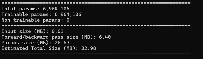

七、总结

7.1 DenseNet121 算法的核心思想是什么？

核心思想 ：密集连接（Dense Connection）与特征重用（Feature Reuse）。
具体表现：它打破了传统网络一层接一层的顺序结构。在一个 Dense Block 中，每一层都会接收前面所有层的输出作为自己的输入（在 Channel 维度上进行拼接 Concat）。这使得特征得到了极致的重复利用，不仅极大减少了参数量，还让梯度回传变得极其顺畅，有效缓解了深层网络的梯度消失问题。

7.2 ResNet 与 DenseNet 的对比

ResNet（上周） ：采用的是相加（Add） 。 X l = H l ( X l − 1 ) + X l − 1 X_l = H_l(X_{l-1}) + X_{l-1} Xl=Hl(Xl−1)+Xl−1。类似于"抄近道"，将信息叠加上去。
DenseNet（本周） ：采用的是拼接（Concat） 。 X l = H l ( [ X 0 , X 1 , . . . , X l − 1 ] ) X_l = H_l([X_0, X_1, ..., X_{l-1}]) Xl=Hl([X0,X1,...,Xl−1])。类似于"滚雪球"，把前面的特征图在厚度（通道）上拼起来，越往后特征越丰富。

7.3 核心网络结构解析

DenseNet121 主要由两个核心组件交替构成：

Dense Block（密集块） ：
- 内部包含多层，每一层都与前面的层密集相连。
- 使用 1x1 卷积（Bottleneck）先降维，再用 3x3 卷积提取特征，以控制计算量。
Transition Layer（过渡层） ：
- 连接在两个 Dense Block 之间。
- 作用是"踩刹车"。因为密集拼接会导致通道数爆炸，过渡层通过 1x1 卷积（减少通道数）和 2x2 平均池化（缩小特征图尺寸），压缩模型大小，提高计算效率。

7.4 实验结果

本周成功将 DenseNet 的结构用 PyTorch 框架进行了复现，并使用 torchsummary 工具打印了模型摘要。

实验结果分析：

总参数量 (Total params) ：约 696 万（6,964,106）。相较于动辄几千万参数的其他模型，DenseNet121 极其轻量化。
内存占用：模型的前向/反向传播占用约 6.40 MB，总预估大小仅 32.98 MB。
结论：充分印证了理论中所说的------DenseNet 通过特征重用，在极少的参数量和计算成本下，实现了强大的特征提取能力。

DenseNet121学习笔记

一、前期准备

二、 定义核心组件：Dense Layer

三、组装：Dense Block

四、过渡组件：Transition Layer（过渡层）

五、 构建完整的 DenseNet 网络

六、运行与模型摘要测试

七、总结

7.1 DenseNet121 算法的核心思想是什么？

7.2 ResNet 与 DenseNet 的对比

7.3 核心网络结构解析

7.4 实验结果

二、定义核心组件：Dense Layer

五、构建完整的 DenseNet 网络