Day 18 编程实战：Keras搭建MLP神经网络

Day 18 编程实战：Keras搭建MLP神经网络

实战目标

1. 掌握Sequential API和Functional API搭建模型
2. 学习模型编译、训练和评估
3. 使用回调函数（EarlyStopping, ModelCheckpoint）
4. 应用Dropout正则化防止过拟合
5. 绘制训练曲线分析模型行为

1. 导入必要的库

import numpy as np
import pandas as pd
import matplotlib.pyplot as plt
import seaborn as sns
import time
import warnings
warnings.filterwarnings('ignore')

from pathlib import Path

# TensorFlow / Keras
import tensorflow as tf
from tensorflow.keras.models import Sequential, Model
from tensorflow.keras.layers import Dense, Dropout, Input, BatchNormalization, Activation
from tensorflow.keras.optimizers import Adam, SGD, RMSprop
from tensorflow.keras.callbacks import (
    EarlyStopping, ModelCheckpoint, ReduceLROnPlateau,
    CSVLogger, TensorBoard
)
from tensorflow.keras.regularizers import l1, l2, l1_l2
from tensorflow.keras.utils import plot_model

# sklearn工具
from sklearn.preprocessing import StandardScaler
from sklearn.model_selection import train_test_split
from sklearn.metrics import (
    accuracy_score, precision_score, recall_score, f1_score,
    roc_auc_score, roc_curve, classification_report, confusion_matrix
)

# 设置随机种子
np.random.seed(42)
tf.random.set_seed(42)

# 预设样式
sns.set_style("whitegrid")
#启用LaTeX渲染（设为False避免LaTeX依赖）
plt.rcParams['text.usetex'] = False
# 设置中文显示
plt.rcParams['font.sans-serif'] = ['Microsoft YaHei', 'DejaVu Sans']
plt.rcParams['axes.unicode_minus'] = False
plt.rcParams['mathtext.fontset'] = 'dejavusans'  # 或 'stix'

print(f"TensorFlow版本: {tf.__version__}")
print(f"CUDA可用: {tf.config.list_physical_devices('GPU')}")

TensorFlow版本: 2.20.0
CUDA可用: []

2. 生成金融数据

def generate_financial_data(ts_code):
    """生成金融数据"""
    
    data_path = Path(r"E:\AppData\quant_trade\klines\kline2014-2024")
    kline_file = data_path / f"{ts_code}.csv"
    
    df = pd.read_csv(kline_file, usecols=["trade_date", "close", "vol"],
                     parse_dates=["trade_date"])\
            .rename(columns={"vol": "volume"})\
            .sort_values(by=["trade_date"])\
            .reset_index(drop=True)
    
    df['return'] = df['close'].pct_change()
    
    # RSI
    delta = df['return'].fillna(0)
    gain = delta.where(delta > 0, 0).rolling(14).mean()
    loss = -delta.where(delta < 0, 0).rolling(14).mean()
    rs = gain / (loss + 1e-10)
    df['rsi'] = 100 - (100 / (1 + rs))
    
    # MACD
    ema12 = df['close'].ewm(span=12, adjust=False).mean()
    ema26 = df['close'].ewm(span=26, adjust=False).mean()
    df['macd'] = ema12 - ema26
    df['macd_signal'] = df['macd'].ewm(span=9, adjust=False).mean()
    
    # 均线比率
    df['ma5'] = df['close'].rolling(5).mean()
    df['ma20'] = df['close'].rolling(20).mean()
    df['ma_ratio'] = df['ma5'] / df['ma20'] - 1
    
    # 波动率
    df['volatility'] = df['return'].rolling(20).std()
    
    # 成交量比率
    df['volume_ratio'] = df['volume'] / df['volume'].rolling(10).mean()
    
    # 动量指标
    for lag in [1, 2, 3, 5, 10]:
        df[f'momentum_{lag}'] = df['return'].shift(lag).fillna(0)
    
    # 目标变量
    df['target'] = (df['return'].shift(-1) > 0).astype(int)
    
    df = df.dropna()
    return df

# 生成数据
ts_code = "300033.SZ"
df = generate_financial_data(ts_code)
print(f"数据形状: {df.shape}")

# 特征选择
feature_cols = ['rsi', 'macd', 'macd_signal', 'ma_ratio', 'volatility', 
                'volume_ratio', 'momentum_1', 'momentum_2', 'momentum_3', 
                'momentum_5', 'momentum_10']
X = df[feature_cols].values
y = df['target'].values

print(f"特征数量: {len(feature_cols)}")
print(f"样本数量: {len(X)}")
print(f"目标分布: {y.mean():.2%}")

# 时间划分
split_idx = int(len(X) * 0.7)
X_train_raw = X[:split_idx]
X_test_raw = X[split_idx:]
y_train = y[:split_idx]
y_test = y[split_idx:]

print(f"\n训练集: {len(X_train_raw)} 样本")
print(f"测试集: {len(X_test_raw)} 样本")

# 标准化
scaler = StandardScaler()
X_train = scaler.fit_transform(X_train_raw)
X_test = scaler.transform(X_test_raw)

# 划分验证集
val_split_idx = int(len(X_train) * 0.8)
X_train_final = X_train[:val_split_idx]
y_train_final = y_train[:val_split_idx]
X_val = X_train[val_split_idx:]
y_val = y_train[val_split_idx:]

print(f"最终训练集: {len(X_train_final)} 样本")
print(f"验证集: {len(X_val)} 样本")

数据形状: (2451, 18)
特征数量: 11
样本数量: 2451
目标分布: 50.43%

训练集: 1715 样本
测试集: 736 样本
最终训练集: 1372 样本
验证集: 343 样本

3. Sequential API搭建MLP

3.1 基础3层MLP

def build_sequential_model(input_dim, dropout_rate=0.0):
    """使用Sequential API构建MLP模型"""
    model = Sequential([
        # 第一隐藏层
        Dense(128, activation='relu', input_shape=(input_dim,)),
        
        # 第二隐藏层
        Dense(64, activation='relu'),
        
        # 第三隐藏层
        Dense(32, activation='relu'),
        
        # 输出层
        Dense(1, activation='sigmoid')
    ])
    
    return model

# 构建模型
input_dim = X_train.shape[1]
model_seq = build_sequential_model(input_dim)

# 查看模型结构
print("模型结构:")
model_seq.summary()

模型结构:

Model: "sequential_3"

┏━━━━━━━━━━━━━━━━━━━━━━━━━━━━━━━━━━━━━━┳━━━━━━━━━━━━━━━━━━━━━━━━━━━━━┳━━━━━━━━━━━━━━━━━┓
┃ Layer (type)                         ┃ Output Shape                ┃         Param # ┃
┡━━━━━━━━━━━━━━━━━━━━━━━━━━━━━━━━━━━━━━╇━━━━━━━━━━━━━━━━━━━━━━━━━━━━━╇━━━━━━━━━━━━━━━━━┩
│ dense_16 (Dense)                     │ (None, 128)                 │           1,536 │
├──────────────────────────────────────┼─────────────────────────────┼─────────────────┤
│ dense_17 (Dense)                     │ (None, 64)                  │           8,256 │
├──────────────────────────────────────┼─────────────────────────────┼─────────────────┤
│ dense_18 (Dense)                     │ (None, 32)                  │           2,080 │
├──────────────────────────────────────┼─────────────────────────────┼─────────────────┤
│ dense_19 (Dense)                     │ (None, 1)                   │              33 │
└──────────────────────────────────────┴─────────────────────────────┴─────────────────┘

 Total params: 11,905 (46.50 KB)

 Trainable params: 11,905 (46.50 KB)

 Non-trainable params: 0 (0.00 B)

3.2 添加Dropout的模型

def build_sequential_with_dropout(input_dim, dropout_rate=0.3):
    """带Dropout的Sequential模型"""
    model = Sequential([
        Dense(128, activation='relu', input_shape=(input_dim,)),
        Dropout(dropout_rate),
        
        Dense(64, activation='relu'),
        Dropout(dropout_rate),
        
        Dense(32, activation='relu'),
        Dropout(dropout_rate * 0.5),
        
        Dense(1, activation='sigmoid')
    ])
    
    return model

model_dropout = build_sequential_with_dropout(input_dim, dropout_rate=0.3)
print("带Dropout的模型:")
model_dropout.summary()

带Dropout的模型:

Model: "sequential_4"

┏━━━━━━━━━━━━━━━━━━━━━━━━━━━━━━━━━━━━━━┳━━━━━━━━━━━━━━━━━━━━━━━━━━━━━┳━━━━━━━━━━━━━━━━━┓
┃ Layer (type)                         ┃ Output Shape                ┃         Param # ┃
┡━━━━━━━━━━━━━━━━━━━━━━━━━━━━━━━━━━━━━━╇━━━━━━━━━━━━━━━━━━━━━━━━━━━━━╇━━━━━━━━━━━━━━━━━┩
│ dense_20 (Dense)                     │ (None, 128)                 │           1,536 │
├──────────────────────────────────────┼─────────────────────────────┼─────────────────┤
│ dropout_6 (Dropout)                  │ (None, 128)                 │               0 │
├──────────────────────────────────────┼─────────────────────────────┼─────────────────┤
│ dense_21 (Dense)                     │ (None, 64)                  │           8,256 │
├──────────────────────────────────────┼─────────────────────────────┼─────────────────┤
│ dropout_7 (Dropout)                  │ (None, 64)                  │               0 │
├──────────────────────────────────────┼─────────────────────────────┼─────────────────┤
│ dense_22 (Dense)                     │ (None, 32)                  │           2,080 │
├──────────────────────────────────────┼─────────────────────────────┼─────────────────┤
│ dropout_8 (Dropout)                  │ (None, 32)                  │               0 │
├──────────────────────────────────────┼─────────────────────────────┼─────────────────┤
│ dense_23 (Dense)                     │ (None, 1)                   │              33 │
└──────────────────────────────────────┴─────────────────────────────┴─────────────────┘

 Total params: 11,905 (46.50 KB)

 Trainable params: 11,905 (46.50 KB)

 Non-trainable params: 0 (0.00 B)

4. Functional API搭建MLP

def build_functional_model(input_dim, dropout_rate=0.0, use_batch_norm=False):
    """使用Functional API构建MLP模型"""
    
    # 输入层
    inputs = Input(shape=(input_dim,))
    
    # 第一隐藏层
    x = Dense(128, activation='relu')(inputs)
    if use_batch_norm:
        x = BatchNormalization()(x)
    if dropout_rate > 0:
        x = Dropout(dropout_rate)(x)
    
    # 第二隐藏层
    x = Dense(64, activation='relu')(x)
    if use_batch_norm:
        x = BatchNormalization()(x)
    if dropout_rate > 0:
        x = Dropout(dropout_rate)(x)
    
    # 第三隐藏层
    x = Dense(32, activation='relu')(x)
    if dropout_rate > 0:
        x = Dropout(dropout_rate * 0.5)(x)
    
    # 输出层
    outputs = Dense(1, activation='sigmoid')(x)
    
    # 创建模型
    model = Model(inputs=inputs, outputs=outputs)
    
    return model

model_func = build_functional_model(input_dim, dropout_rate=0.2)
print("Functional API模型:")
model_func.summary()

Functional API模型:

Model: "functional_6"

┏━━━━━━━━━━━━━━━━━━━━━━━━━━━━━━━━━━━━━━┳━━━━━━━━━━━━━━━━━━━━━━━━━━━━━┳━━━━━━━━━━━━━━━━━┓
┃ Layer (type)                         ┃ Output Shape                ┃         Param # ┃
┡━━━━━━━━━━━━━━━━━━━━━━━━━━━━━━━━━━━━━━╇━━━━━━━━━━━━━━━━━━━━━━━━━━━━━╇━━━━━━━━━━━━━━━━━┩
│ input_layer_6 (InputLayer)           │ (None, 11)                  │               0 │
├──────────────────────────────────────┼─────────────────────────────┼─────────────────┤
│ dense_24 (Dense)                     │ (None, 128)                 │           1,536 │
├──────────────────────────────────────┼─────────────────────────────┼─────────────────┤
│ dropout_9 (Dropout)                  │ (None, 128)                 │               0 │
├──────────────────────────────────────┼─────────────────────────────┼─────────────────┤
│ dense_25 (Dense)                     │ (None, 64)                  │           8,256 │
├──────────────────────────────────────┼─────────────────────────────┼─────────────────┤
│ dropout_10 (Dropout)                 │ (None, 64)                  │               0 │
├──────────────────────────────────────┼─────────────────────────────┼─────────────────┤
│ dense_26 (Dense)                     │ (None, 32)                  │           2,080 │
├──────────────────────────────────────┼─────────────────────────────┼─────────────────┤
│ dropout_11 (Dropout)                 │ (None, 32)                  │               0 │
├──────────────────────────────────────┼─────────────────────────────┼─────────────────┤
│ dense_27 (Dense)                     │ (None, 1)                   │              33 │
└──────────────────────────────────────┴─────────────────────────────┴─────────────────┘

 Total params: 11,905 (46.50 KB)

 Trainable params: 11,905 (46.50 KB)

 Non-trainable params: 0 (0.00 B)

5. 模型编译与训练

5.1 编译配置

def compile_model(model, learning_rate=0.001, optimizer='adam'):
    """编译模型"""
    
    if optimizer == 'adam':
        opt = Adam(learning_rate=learning_rate)
    elif optimizer == 'sgd':
        opt = SGD(learning_rate=learning_rate, momentum=0.9)
    elif optimizer == 'rmsprop':
        opt = RMSprop(learning_rate=learning_rate)
    else:
        opt = optimizer
    
    model.compile(
        optimizer=opt,
        loss='binary_crossentropy',
        metrics=['accuracy']
    )
    
    return model

# 编译模型
model_seq = compile_model(model_seq, learning_rate=0.001, optimizer='adam')
print("模型编译完成")

模型编译完成

5.2 配置回调函数

def create_callbacks(model_name='best_model', patience=10):
    """创建训练回调函数"""
    
    callbacks = []
    
    # 1. Early Stopping
    early_stop = EarlyStopping(
        monitor='val_loss',
        patience=patience,
        min_delta=1e-4,
        restore_best_weights=True,
        verbose=1
    )
    callbacks.append(early_stop)
    
    # 2. Model Checkpoint
    checkpoint = ModelCheckpoint(
        f'{model_name}_checkpoint.keras',
        monitor='val_accuracy',
        save_best_only=True,
        save_weights_only=False,
        mode='max',
        verbose=0
    )
    callbacks.append(checkpoint)
    
    # 3. Reduce LR on Plateau
    reduce_lr = ReduceLROnPlateau(
        monitor='val_loss',
        factor=0.5,
        patience=5,
        min_lr=1e-6,
        verbose=0
    )
    callbacks.append(reduce_lr)
    
    return callbacks

# 创建回调
callbacks = create_callbacks(model_name='mlp_model', patience=10)

5.3 训练模型

print("="*60)
print("开始训练模型")
print("="*60)

start_time = time.time()

history = model_seq.fit(
    X_train_final, y_train_final,
    epochs=100,
    batch_size=32,
    validation_data=(X_val, y_val),
    callbacks=callbacks,
    verbose=1
)

train_time = time.time() - start_time
print(f"\n训练完成，耗时: {train_time:.2f}秒")

============================================================
开始训练模型
============================================================
Epoch 1/100
[1m43/43[0m [32m━━━━━━━━━━━━━━━━━━━━[0m[37m[0m [1m0s[0m 5ms/step - accuracy: 0.6698 - loss: 0.6322 - val_accuracy: 0.6093 - val_loss: 0.6669 - learning_rate: 2.5000e-04
Epoch 2/100
[1m43/43[0m [32m━━━━━━━━━━━━━━━━━━━━[0m[37m[0m [1m0s[0m 3ms/step - accuracy: 0.6698 - loss: 0.6299 - val_accuracy: 0.6035 - val_loss: 0.6668 - learning_rate: 2.5000e-04
Epoch 3/100
[1m43/43[0m [32m━━━━━━━━━━━━━━━━━━━━[0m[37m[0m [1m0s[0m 3ms/step - accuracy: 0.6713 - loss: 0.6277 - val_accuracy: 0.6035 - val_loss: 0.6670 - learning_rate: 2.5000e-04
Epoch 4/100
[1m43/43[0m [32m━━━━━━━━━━━━━━━━━━━━[0m[37m[0m [1m0s[0m 3ms/step - accuracy: 0.6749 - loss: 0.6256 - val_accuracy: 0.6006 - val_loss: 0.6671 - learning_rate: 2.5000e-04
Epoch 5/100
[1m43/43[0m [32m━━━━━━━━━━━━━━━━━━━━[0m[37m[0m [1m0s[0m 3ms/step - accuracy: 0.6778 - loss: 0.6237 - val_accuracy: 0.5948 - val_loss: 0.6674 - learning_rate: 2.5000e-04
Epoch 6/100
[1m43/43[0m [32m━━━━━━━━━━━━━━━━━━━━[0m[37m[0m [1m0s[0m 3ms/step - accuracy: 0.6764 - loss: 0.6217 - val_accuracy: 0.5948 - val_loss: 0.6677 - learning_rate: 2.5000e-04
Epoch 7/100
[1m43/43[0m [32m━━━━━━━━━━━━━━━━━━━━[0m[37m[0m [1m0s[0m 3ms/step - accuracy: 0.6771 - loss: 0.6189 - val_accuracy: 0.5918 - val_loss: 0.6675 - learning_rate: 1.2500e-04
Epoch 8/100
[1m43/43[0m [32m━━━━━━━━━━━━━━━━━━━━[0m[37m[0m [1m0s[0m 3ms/step - accuracy: 0.6800 - loss: 0.6178 - val_accuracy: 0.5918 - val_loss: 0.6679 - learning_rate: 1.2500e-04
Epoch 9/100
[1m43/43[0m [32m━━━━━━━━━━━━━━━━━━━━[0m[37m[0m [1m0s[0m 3ms/step - accuracy: 0.6815 - loss: 0.6167 - val_accuracy: 0.5918 - val_loss: 0.6682 - learning_rate: 1.2500e-04
Epoch 10/100
[1m43/43[0m [32m━━━━━━━━━━━━━━━━━━━━[0m[37m[0m [1m0s[0m 3ms/step - accuracy: 0.6829 - loss: 0.6156 - val_accuracy: 0.5918 - val_loss: 0.6684 - learning_rate: 1.2500e-04
Epoch 11/100
[1m43/43[0m [32m━━━━━━━━━━━━━━━━━━━━[0m[37m[0m [1m1s[0m 10ms/step - accuracy: 0.6837 - loss: 0.6145 - val_accuracy: 0.5948 - val_loss: 0.6687 - learning_rate: 1.2500e-04
Epoch 11: early stopping
Restoring model weights from the end of the best epoch: 1.

训练完成，耗时: 2.63秒

5.4 绘制训练曲线

def plot_training_history(history, title="训练曲线"):
    """绘制训练损失和准确率曲线"""
    
    fig, axes = plt.subplots(1, 2, figsize=(14, 5))
    
    # 损失曲线
    axes[0].plot(history.history['loss'], 'b-', label='训练损失', linewidth=2)
    axes[0].plot(history.history['val_loss'], 'r-', label='验证损失', linewidth=2)
    axes[0].set_xlabel('Epoch')
    axes[0].set_ylabel('损失')
    axes[0].set_title('训练 vs 验证损失')
    axes[0].legend()
    axes[0].grid(True, alpha=0.3)
    
    # 准确率曲线
    axes[1].plot(history.history['accuracy'], 'b-', label='训练准确率', linewidth=2)
    axes[1].plot(history.history['val_accuracy'], 'r-', label='验证准确率', linewidth=2)
    axes[1].set_xlabel('Epoch')
    axes[1].set_ylabel('准确率')
    axes[1].set_title('训练 vs 验证准确率')
    axes[1].legend()
    axes[1].grid(True, alpha=0.3)
    
    plt.suptitle(title, fontsize=14)
    plt.tight_layout()
    plt.show()
    
    # 打印最佳结果
    best_epoch = np.argmin(history.history['val_loss']) + 1
    best_val_loss = min(history.history['val_loss'])
    best_val_acc = max(history.history['val_accuracy'])
    
    print(f"最佳轮数: {best_epoch}")
    print(f"最佳验证损失: {best_val_loss:.4f}")
    print(f"最佳验证准确率: {best_val_acc:.4f}")

plot_training_history(history, "基础3层MLP训练曲线")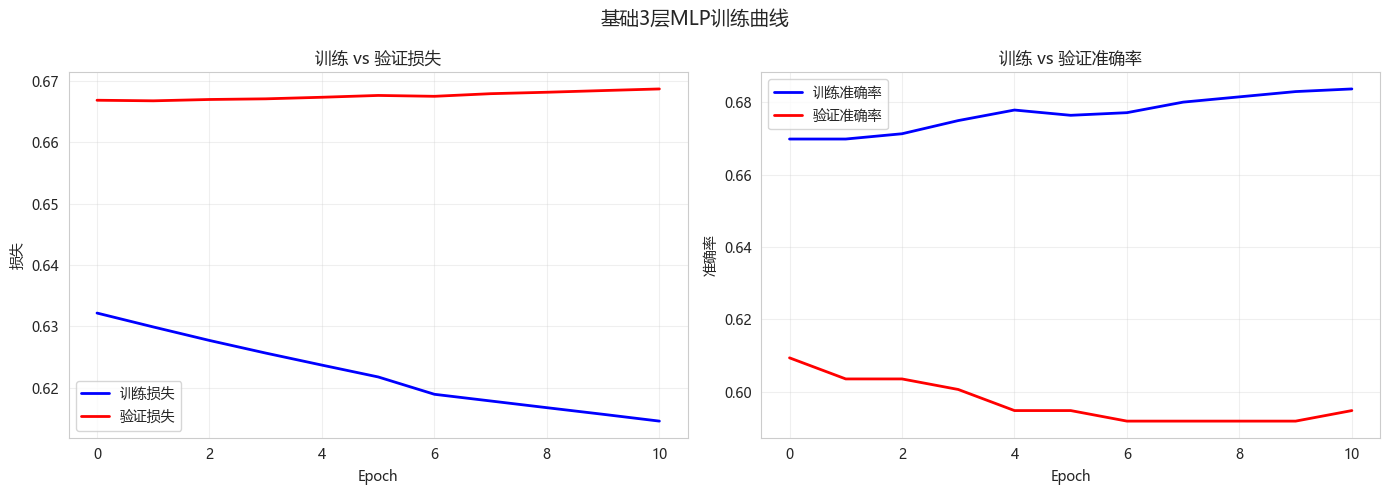

最佳轮数: 2
最佳验证损失: 0.6668
最佳验证准确率: 0.6093

6. 模型评估

6.1 测试集评估

# 预测
y_pred_proba = model_seq.predict(X_test)
y_pred = (y_pred_proba > 0.5).astype(int)

# 评估指标
print("="*60)
print("测试集评估结果")
print("="*60)

print(f"准确率: {accuracy_score(y_test, y_pred):.4f}")
print(f"精确率: {precision_score(y_test, y_pred):.4f}")
print(f"召回率: {recall_score(y_test, y_pred):.4f}")
print(f"F1分数: {f1_score(y_test, y_pred):.4f}")
print(f"AUC: {roc_auc_score(y_test, y_pred_proba):.4f}")

# 混淆矩阵
cm = confusion_matrix(y_test, y_pred)
plt.figure(figsize=(8, 6))
sns.heatmap(cm, annot=True, fmt='d', cmap='Blues',
            xticklabels=['下跌', '上涨'], yticklabels=['下跌', '上涨'])
plt.title('混淆矩阵')
plt.xlabel('预测')
plt.ylabel('真实')
plt.show()

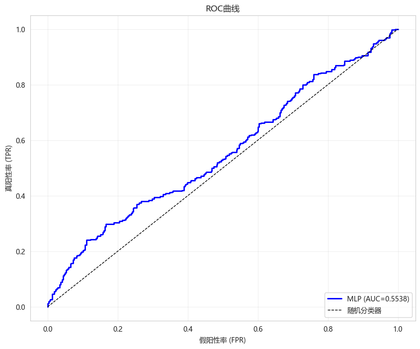
# ROC曲线
fpr, tpr, _ = roc_curve(y_test, y_pred_proba)
auc = roc_auc_score(y_test, y_pred_proba)

plt.figure(figsize=(10, 8))
plt.plot(fpr, tpr, 'b-', linewidth=2, label=f'MLP (AUC={auc:.4f})')
plt.plot([0, 1], [0, 1], 'k--', linewidth=1, label='随机分类器')
plt.xlabel('假阳性率 (FPR)')
plt.ylabel('真阳性率 (TPR)')
plt.title('ROC曲线')
plt.legend(loc='lower right')
plt.grid(True, alpha=0.3)
plt.show()

[1m23/23[0m [32m━━━━━━━━━━━━━━━━━━━━[0m[37m[0m [1m0s[0m 2ms/step  
============================================================
测试集评估结果
============================================================
准确率: 0.5136
精确率: 0.4904
召回率: 0.5829
F1分数: 0.5326
AUC: 0.5538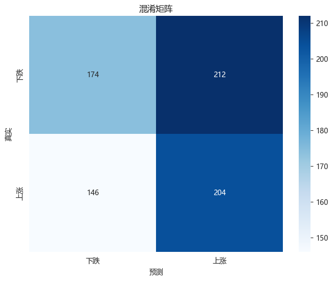

7. Dropout防过拟合效果对比

7.1 训练两个模型对比

print("="*60)
print("对比实验：无Dropout vs 有Dropout")
print("="*60)

# 无Dropout模型
model_no_dropout = build_sequential_model(input_dim)
model_no_dropout = compile_model(model_no_dropout)
callbacks_no_dropout = create_callbacks(model_name='no_dropout', patience=10)

history_no_dropout = model_no_dropout.fit(
    X_train_final, y_train_final,
    epochs=100,
    batch_size=32,
    validation_data=(X_val, y_val),
    callbacks=callbacks_no_dropout,
    verbose=0
)

# 有Dropout模型
model_with_dropout = build_sequential_with_dropout(input_dim, dropout_rate=0.3)
model_with_dropout = compile_model(model_with_dropout)
callbacks_dropout = create_callbacks(model_name='with_dropout', patience=10)

history_with_dropout = model_with_dropout.fit(
    X_train_final, y_train_final,
    epochs=100,
    batch_size=32,
    validation_data=(X_val, y_val),
    callbacks=callbacks_dropout,
    verbose=0
)

# 测试集评估
y_pred_no = (model_no_dropout.predict(X_test) > 0.5).astype(int)
y_pred_with = (model_with_dropout.predict(X_test) > 0.5).astype(int)

print(f"\n{'配置':<15} {'训练准确率':<12} {'验证准确率':<12} {'测试准确率':<12} {'过拟合差距':<12}")
print("-"*63)

train_acc_no = max(history_no_dropout.history['accuracy'])
val_acc_no = max(history_no_dropout.history['val_accuracy'])
test_acc_no = accuracy_score(y_test, y_pred_no)
gap_no = train_acc_no - val_acc_no

train_acc_with = max(history_with_dropout.history['accuracy'])
val_acc_with = max(history_with_dropout.history['val_accuracy'])
test_acc_with = accuracy_score(y_test, y_pred_with)
gap_with = train_acc_with - val_acc_with

print(f"{'无Dropout':<15} {train_acc_no:<12.4f} {val_acc_no:<12.4f} {test_acc_no:<12.4f} {gap_no:<12.4f}")
print(f"{'有Dropout':<15} {train_acc_with:<12.4f} {val_acc_with:<12.4f} {test_acc_with:<12.4f} {gap_with:<12.4f}")

# 损失曲线对比
fig, axes = plt.subplots(1, 2, figsize=(14, 5))

axes[0].plot(history_no_dropout.history['val_loss'], 'b-', label='无Dropout', linewidth=2)
axes[0].plot(history_with_dropout.history['val_loss'], 'r-', label='有Dropout', linewidth=2)
axes[0].set_xlabel('Epoch')
axes[0].set_ylabel('验证损失')
axes[0].set_title('验证损失对比')
axes[0].legend()
axes[0].grid(True, alpha=0.3)

axes[1].plot(history_no_dropout.history['val_accuracy'], 'b-', label='无Dropout', linewidth=2)
axes[1].plot(history_with_dropout.history['val_accuracy'], 'r-', label='有Dropout', linewidth=2)
axes[1].set_xlabel('Epoch')
axes[1].set_ylabel('验证准确率')
axes[1].set_title('验证准确率对比')
axes[1].legend()
axes[1].grid(True, alpha=0.3)

plt.suptitle('Dropout正则化效果对比', fontsize=14)
plt.tight_layout()
plt.show()

============================================================
对比实验：无Dropout vs 有Dropout
============================================================
Epoch 18: early stopping
Restoring model weights from the end of the best epoch: 8.
Epoch 21: early stopping
Restoring model weights from the end of the best epoch: 11.
[1m23/23[0m [32m━━━━━━━━━━━━━━━━━━━━[0m[37m[0m [1m0s[0m 1ms/step 
[1m23/23[0m [32m━━━━━━━━━━━━━━━━━━━━[0m[37m[0m [1m0s[0m 1ms/step 

配置              训练准确率        验证准确率        测试准确率        过拟合差距       
---------------------------------------------------------------
无Dropout        0.7726       0.5860       0.5109       0.1866      
有Dropout        0.6181       0.6152       0.5367       0.0029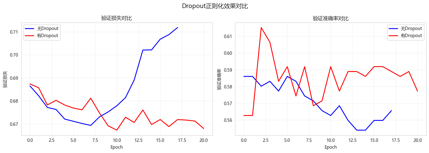      

8. 超参数搜索实验

8.1 不同隐藏层大小对比

def experiment_hidden_layers(X_train, X_val, y_train, y_val, X_test, y_test):
    """实验不同隐藏层配置"""
    
    hidden_configs = [
        (64, 32),
        (128, 64),
        (256, 128),
        (128, 64, 32),
        (256, 128, 64)
    ]
    
    results = []
    
    for config in hidden_configs:
        # 构建模型
        model = Sequential()
        model.add(Dense(config[0], activation='relu', input_shape=(X_train.shape[1],)))
        model.add(Dropout(0.3))
        
        for units in config[1:]:
            model.add(Dense(units, activation='relu'))
            model.add(Dropout(0.3))
        
        model.add(Dense(1, activation='sigmoid'))
        
        model.compile(optimizer='adam', loss='binary_crossentropy', metrics=['accuracy'])
        
        early_stop = EarlyStopping(monitor='val_loss', patience=10, restore_best_weights=True)
        
        history = model.fit(
            X_train, y_train,
            epochs=100,
            batch_size=32,
            validation_data=(X_val, y_val),
            callbacks=[early_stop],
            verbose=0
        )
        
        y_pred_proba = model.predict(X_test, verbose=0)
        auc = roc_auc_score(y_test, y_pred_proba)
        
        results.append({
            '隐藏层配置': str(config),
            '最佳验证准确率': max(history.history['val_accuracy']),
            'AUC': auc,
            '训练轮数': len(history.history['loss'])
        })
    
    return pd.DataFrame(results)

print("开始隐藏层大小实验...")
hidden_results = experiment_hidden_layers(
    X_train_final, X_val, y_train_final, y_val, X_test, y_test
)
print(hidden_results.to_string(index=False))

开始隐藏层大小实验...
         隐藏层配置  最佳验证准确率      AUC  训练轮数
      (64, 32) 0.606414 0.559423    48
     (128, 64) 0.603499 0.564256    17
    (256, 128) 0.597668 0.558357    22
 (128, 64, 32) 0.594752 0.565174    39
(256, 128, 64) 0.618076 0.565699    27

8.2 不同Dropout率对比

def experiment_dropout_rates(X_train, X_val, y_train, y_val, X_test, y_test):
    """实验不同Dropout率"""
    
    dropout_rates = [0.0, 0.1, 0.2, 0.3, 0.4, 0.5]
    results = []
    
    for dr in dropout_rates:
        model = Sequential([
            Dense(128, activation='relu', input_shape=(X_train.shape[1],)),
            Dropout(dr),
            Dense(64, activation='relu'),
            Dropout(dr),
            Dense(32, activation='relu'),
            Dropout(dr * 0.5),
            Dense(1, activation='sigmoid')
        ])
        
        model.compile(optimizer='adam', loss='binary_crossentropy', metrics=['accuracy'])
        
        early_stop = EarlyStopping(monitor='val_loss', patience=10, restore_best_weights=True)
        
        history = model.fit(
            X_train, y_train,
            epochs=100,
            batch_size=32,
            validation_data=(X_val, y_val),
            callbacks=[early_stop],
            verbose=0
        )
        
        y_pred_proba = model.predict(X_test, verbose=0)
        auc = roc_auc_score(y_test, y_pred_proba)
        
        # 计算过拟合程度
        train_acc = max(history.history['accuracy'])
        val_acc = max(history.history['val_accuracy'])
        
        results.append({
            'Dropout率': dr,
            'AUC': auc,
            '训练准确率': train_acc,
            '验证准确率': val_acc,
            '过拟合差距': train_acc - val_acc
        })
    
    return pd.DataFrame(results)

print("开始Dropout率实验...")
dropout_results = experiment_dropout_rates(
    X_train_final, X_val, y_train_final, y_val, X_test, y_test
)
print(dropout_results.to_string(index=False))

# 可视化
plt.figure(figsize=(12, 5))

plt.subplot(1, 2, 1)
plt.plot(dropout_results['Dropout率'], dropout_results['AUC'], 'bo-', linewidth=2)
plt.xlabel('Dropout率')
plt.ylabel('AUC')
plt.title('Dropout率对AUC的影响')
plt.grid(True, alpha=0.3)

plt.subplot(1, 2, 2)
plt.plot(dropout_results['Dropout率'], dropout_results['过拟合差距'], 'ro-', linewidth=2)
plt.xlabel('Dropout率')
plt.ylabel('过拟合差距(训练-验证)')
plt.title('Dropout率对过拟合的影响')
plt.grid(True, alpha=0.3)

plt.suptitle('Dropout率实验', fontsize=14)
plt.tight_layout()
plt.show()

开始Dropout率实验...
 Dropout率      AUC    训练准确率    验证准确率    过拟合差距
      0.0 0.558046 0.742711 0.612245 0.130466
      0.1 0.556454 0.697522 0.615160 0.082362
      0.2 0.559911 0.637755 0.597668 0.040087
      0.3 0.564589 0.617347 0.603499 0.013848
      0.4 0.563967 0.629738 0.612245 0.017493
      0.5 0.573472 0.644315 0.594752 0.049563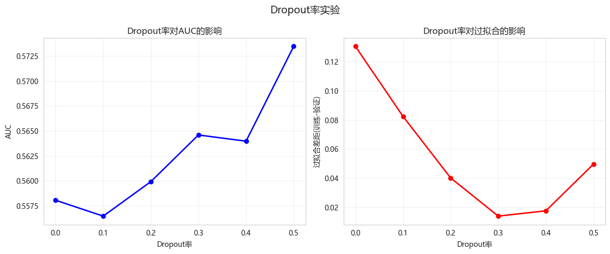

9. 模型保存与加载

9.1 保存模型

# 保存整个模型
best_model = model_with_dropout
best_model.save('best_mlp.model.keras')
print("模型已保存为 best_mlp.model.keras")

# 仅保存权重
best_model.save_weights('best_mlp.weights.h5')
print("模型权重已保存为 best_mlp.weights.h5")

模型已保存为 best_mlp.model.keras
模型权重已保存为 best_mlp.weights.h5

9.2 加载模型

from tensorflow.keras.models import load_model

# 加载整个模型
loaded_model = load_model('best_mlp.model.keras')
print("模型加载成功")

# 验证加载的模型
y_pred_loaded = loaded_model.predict(X_test)
print(f"加载模型AUC: {roc_auc_score(y_test, y_pred_loaded):.4f}")
print(f"原模型AUC: {roc_auc_score(y_test, best_model.predict(X_test)):.4f}")

模型加载成功
[1m23/23[0m [32m━━━━━━━━━━━━━━━━━━━━[0m[37m[0m [1m0s[0m 2ms/step 
加载模型AUC: 0.5708
[1m23/23[0m [32m━━━━━━━━━━━━━━━━━━━━[0m[37m[0m [1m0s[0m 1ms/step 
原模型AUC: 0.5708

10. 今日总结

1. Keras核心组件：

   • Sequential API: 简单线性堆叠
   • Functional API: 复杂拓扑结构
   • 层(Dense)、激活函数、优化器、损失函数

2. 回调函数应用：

   • EarlyStopping: 防止过拟合，自动停止训练
   • ModelCheckpoint: 保存最佳模型# - ReduceLROnPlateau: 自适应学习率衰减

3. Dropout正则化效果：

   • 无Dropout: 训练准确率={train_acc_no:.4f}, 验证准确率={val_acc_no:.4f}, 差距={gap_no:.4f}
   • 有Dropout: 训练准确率={train_acc_with:.4f}, 验证准确率={val_acc_with:.4f}, 差距={gap_with:.4f}
   • Dropout有效减少了过拟合！

4. 最佳Dropout率: 0.5

5. 量化应用建议：

   • 神经网络适合非线性关系复杂的场景
   • 使用EarlyStopping防止过拟合
   • 验证集表现比训练集表现更重要
   • 可使用ModelCheckpoint保存最佳模型

6. 扩展作业

   • 作业1：尝试不同的优化器（Adam, SGD, RMSprop），对比收敛速度
   • 作业2：实现学习率调度器（学习率随epoch衰减）
   • 作业3：使用Functional API搭建多输入网络（如技术指标+基本面数据）
   • 作业4：实现自定义回调函数（如每5轮打印学习率）

7. 今日收获（3个）

   1. 掌握了Sequential和Functional API搭建模型
   2. 学会了使用回调函数进行训练控制
   3. 理解了Dropout正则化的作用

8. 量化思考

   • Keras提供了方便的API来构建深度学习模型
   • Dropout和EarlyStopping是防止过拟合的有效手段
   • 训练曲线可以帮助诊断欠拟合/过拟合
   • 始终使用验证集来评估模型泛化能力

9. 常见错误排查指南

   • 问题1: Loss不下降
     • 检查数据是否标准化
     • 降低学习率
     • 增加网络容量
   • 问题2: 训练集Loss下降但验证集不下降（过拟合）
     • 增加Dropout率
     • 添加L2正则化
     • 减少网络容量
     • 使用EarlyStopping
   • 问题3: 训练Loss震荡
     • 降低学习率
     • 增大batch_size
     • 使用学习率调度
   • 问题4: 验证集Loss比训练集低
     • 通常正常（Dropout导致）
     • 检查数据泄露