1.作者介绍
任鑫,男,西安工程大学电子信息学院,2025级研究生
研究方向:深度学习、目标检测
电子邮件:renx17811@163.com
胥乾信,男,西安工程大学电子信息学院,2025级研究生,张宏伟人工智能课题组
研究方向:机器视觉与人工智能
电子邮件:2692797728@qq.com
2.弹性网络回归(Elastic Net Regression)介绍
2.1 回归与正则化基础
线性回归的本质是找到特征与目标值的线性映射关系,公式为:

模型训练的目标是找到最优的w和b,让预测值与真实值的均方误差(MSE)最小。
2.2弹性网络回归的数学原理
普通线性回归易出现过拟合和多重共线性问题,因此引入L1、L2两种正则化,二者作用互补:既实现特征选择(L1正则化),又处理多重共线性(L2正则化),兼顾模型的稀疏性和稳定性。
1)弹性网络回归的损失函数是数据误差项+L1正则化项+L2正则化项的组合,标准形式为:

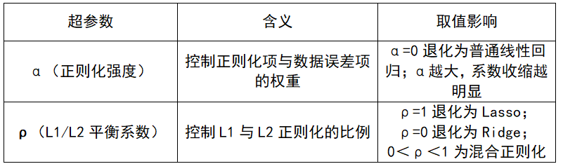
2)有两个核心的超参数:
3)模型的优化目标:
弹性网络回归的本质是带约束的凸优化问题,目标是找到最优的回归系数w,让损失函数最小:

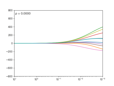
图1 不同的ρ对弹性网络回归的影响
当ρ逐渐增大时,L1正则项占据主导地位,代价函数越接近Lasso回归;ρ逐渐减小时,L2正则项占据主导地位,代价函数越接近Ridge回归。
2.3 弹性网络回归的求解方法
由于L1正则化项的存在,损失函数在 处不可导,因此无法直接用普通梯度下降法求解,常用两种优化方法。
2.4弹性网络回归的案例
1)预测水果店供应商综合满意度
有价格(x1)、配送时间(x2)、水果质量(x3)3个特征,预测供应商的综合满意度(y,1-10分)。
单一正则化的问题:用Lasso:可能随机将"配送时间"的系数压缩为0,丢失重要特征;用Ridge:保留所有3个特征,若存在冗余特征(如后续加入"运费",与价格高度相关),模型会冗余。
弹性网络的优势:既会将真正无关的特征(如后续加入的"供应商名称")系数压缩为0,又会对高度相关的特征(价格、运费)做系数平滑,让模型既稀疏又稳定。
2)使用模拟高维数据集(500样本+10特征)进行弹性网络回归,步骤包括:数据生成、预处理、建模、评估、可视化。
图3 模拟高维数据集可视化图
3.基于ElasticNet网格搜索的汽车燃油效率预测
3.1 Auto MPG数据集
MPG汽车油耗数据集源自1983年的美国统计协会博览会,包含398个样本,9个特征,用于回归任务。
使用Seaborn的MPG数据集:https://raw.githubusercontent.com/mwaskom/seaborn-data/master/mpg.csv
Github链接:seaborn-data/mpg.csv at master · mwaskom/seaborn-data
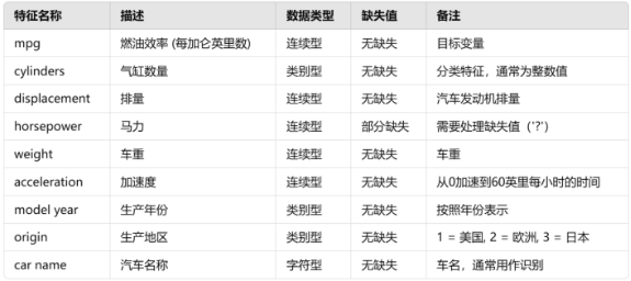
图4 数据集介绍
3.2 代码调试
1)导入必要库
python
import numpy as np
import pandas as pd
import matplotlib.pyplot as plt
import seaborn as sns
# 导入数据集生成、模型、评估指标、数据处理工具
from sklearn.datasets import make_regression
from sklearn.model_selection import train_test_split, GridSearchCV
from sklearn.preprocessing import StandardScaler
from sklearn.linear_model import ElasticNet
from sklearn.metrics import r2_score, mean_squared_error
import urllib.request
import os
2)加载Auto MPG数据集
python
try:
    # 直接从GitHub加载数据
    github_url = 'https://raw.githubusercontent.com/mwaskom/seaborn-data/master/mpg.csv'
    data = pd.read_csv(github_url)
    print("成功从GitHub加载MPG数据集")
    print(f"原始数据形状: {data.shape}")
    print(f"数据列: {list(data.columns)}")
except:
    print("无法从GitHub加载数据,正在使用模拟数据")
    # 如果无法获取真实数据,则生成模拟数据作为备用
    X_sim, y_sim, coef_sim = make_regression(n_samples=400, n_features=7, noise=10, random_state=42, coef=True)
    # 创建模拟数据框,对应MPG数据集的特征
    sim_columns = ["cylinders", "displacement", "horsepower", "weight", "acceleration", "model_year", "origin","name"]
    data = pd.DataFrame(X_sim, columns=sim_columns)
    data['mpg'] = y_sim

# 数据预处理
print("\n数据预处理开始...")

# 查看缺失值情况
print(f"缺失值统计:\n{data.isnull().sum()}")

# 删除含有缺失值的行(主要针对horsepower列)
data = data.dropna()

# 查看数据类型
print(f"\n数据类型:\n{data.dtypes}")

# 查看分类列的唯一值
print(f"\norigin列的唯一值: {data['origin'].unique()}")
if 'country' in data.columns:
    print(f"country列的唯一值: {data['country'].unique()}")

# 处理分类变量 - 对origin列进行独热编码
origin_encoded = pd.get_dummies(data['origin'], prefix='origin')
print(f"独热编码后的origin列: {list(origin_encoded.columns)}")

# 合并独热编码后的origin列和原始数据
data_processed = pd.concat([data, origin_encoded], axis=1)

# 选择数值型特征用于建模(排除原始的分类列)
feature_cols = []
for col in ['cylinders', 'displacement', 'horsepower', 'weight', 'acceleration', 'model_year',
            'origin_1', 'origin_2', 'origin_3']:  # 包含独热编码后的origin列
    if col in data_processed.columns:
        feature_cols.append(col)

X = data_processed[feature_cols]
y = data_processed['mpg']

print(f"处理后数据形状: {X.shape}")
print(f"特征列: {list(X.columns)}")
print(f"前5行数据:\n{X.head()}")

# 确保所有特征列都是数值型
for col in X.columns:
    X[col] = pd.to_numeric(X[col], errors='coerce')

# 再次删除可能产生的NaN值
data_clean = pd.concat([X, y], axis=1).dropna()
X = data_clean[X.columns]
y = data_clean['mpg']

print(f"清理后数据形状: {X.shape}")
3)数据预处理
python
# 1. 划分训练集(80%)和测试集(20%)
X_train, X_test, y_train, y_test = train_test_split(
    X, y, test_size=0.2, random_state=42
)

# 2. 特征标准化(正则化回归模型必做,消除量纲影响)
scaler = StandardScaler()
X_train_scaled = scaler.fit_transform(X_train)  # 训练集拟合+转换
X_test_scaled = scaler.transform(X_test)        # 测试集仅转换,避免数据泄露

print(f"训练集形状: {X_train_scaled.shape}")
print(f"测试集形状: {X_test_scaled.shape}")
4)使用网格搜索优化弹性网络回归模型
python
# 定义超参数搜索空间
param_grid = {
    'alpha': [0.001, 0.01, 0.1, 1, 10, 100],    #α值,控制正则化强度,越大正则化越强
    'l1_ratio': [0.1, 0.3, 0.5, 0.7, 0.9]      #ρ值,控制L1和L2的权重
}
# 创建ElasticNet模型
elastic_net = ElasticNet(random_state=42)

# 使用网格搜索寻找最佳参数
grid_search = GridSearchCV(
    estimator=elastic_net,
    param_grid=param_grid,
    cv=5,  # 5折交叉验证
    scoring='r2',  # 使用R²作为评分标准
    n_jobs=-1,  # 使用所有CPU核心
    verbose=1   # 显示进度`在这里插入代码片`
)

print("开始网格搜索...")
grid_search.fit(X_train_scaled, y_train)  # 执行网格搜索

# 获取最佳模型和参数
best_elastic_net = grid_search.best_estimator_
best_params = grid_search.best_params_

print(f"最佳参数: {best_params}")
print(f"最佳交叉验证得分: {grid_search.best_score_:.4f}")
5)模型预测与评估
python
# 对训练集和测试集进行预测
y_pred_train = best_elastic_net.predict(X_train_scaled)
y_pred_test = best_elastic_net.predict(X_test_scaled)

# 计算评估指标:R²(越接近1越好)、MSE(越小越好)
r2_train = r2_score(y_train, y_pred_train)
r2_test = r2_score(y_test, y_pred_test)
mse_train = mean_squared_error(y_train, y_pred_train)
mse_test = mean_squared_error(y_test, y_pred_test)

# 输出评估结果
print("========== 弹性网络回归模型性能 ==========")
print(f"最佳参数: {best_params}")
print(f"训练集R²:{r2_train:.4f},训练集MSE:{mse_train:.4f}")
print(f"测试集R²:{r2_test:.4f},测试集MSE:{mse_test:.4f}")

# 比较网格搜索前后的性能(使用默认参数)
default_elastic_net = ElasticNet(alpha=0.1, l1_ratio=0.5, random_state=42)
default_elastic_net.fit(X_train_scaled, y_train)
y_pred_default_test = default_elastic_net.predict(X_test_scaled)
r2_default_test = r2_score(y_test, y_pred_default_test)
mse_default_test = mean_squared_error(y_test, y_pred_default_test)

print(f"\n默认参数模型测试集R²:{r2_default_test:.4f},MSE:{mse_default_test:.4f}")
print(f"网格搜索提升: R² 提升 {r2_test - r2_default_test:.4f}, MSE 改善 {mse_default_test - mse_test:.4f}")
6)多维度可视化分析
python
plt.figure(figsize=(15, 10))  # 设置画布大小

# 子图1:特征重要性(回归系数值,系数为0表示被筛选掉)
plt.subplot(2, 2, 1)
coef = best_elastic_net.coef_  # 获取回归系数
colors = sns.color_palette("coolwarm", len(coef))
plt.barh(range(len(X.columns)), coef, color=colors)
plt.yticks(range(len(X.columns)), X.columns)
plt.title('Feature Importance (ElasticNet Coefficients)', fontsize=16)
plt.xlabel('Coefficient Value', fontsize=12)
plt.ylabel('Feature', fontsize=12)

# 添加网格线以便更好地读取数值
plt.grid(axis='x', linestyle='--', alpha=0.6)

# 子图2:测试集真实值 vs 预测值(点越靠近红线,拟合效果越好)
plt.subplot(2, 2, 2)
plt.scatter(y_test, y_pred_test, c=y_pred_test, cmap='cool', alpha=0.7, edgecolor='k')
plt.plot([min(y_test), max(y_test)], [min(y_test), max(y_test)], color='red', linewidth=2)
plt.title('Predicted vs True Values', fontsize=16)
plt.xlabel('True Values', fontsize=12)
plt.ylabel('Predicted Values', fontsize=12)
plt.colorbar(label="Predicted Value Intensity")

# 子图3:残差分布(残差=真实值-预测值,越靠近0线,模型越稳定)
plt.subplot(2, 2, 3)
residuals = y_test - y_pred_test
plt.scatter(y_pred_test, residuals, c=residuals, cmap='Spectral', alpha=0.7, edgecolor='k')
plt.axhline(y=0, color='red', linestyle='--', linewidth=2)
plt.title('Residuals vs Predicted Values', fontsize=16)
plt.xlabel('Predicted Values', fontsize=12)
plt.ylabel('Residuals', fontsize=12)
plt.colorbar(label="Residual Intensity")

# 子图4:模型性能指标对比(训练集vs测试集)
plt.subplot(2, 2, 4)
metrics = ['Train R²', 'Test R²', 'Train MSE', 'Test MSE']
values = [r2_train, r2_test, mse_train, mse_test]
colors = sns.color_palette("viridis", len(metrics))
bars = plt.bar(metrics, values, color=colors)
plt.title('Model Performance Metrics', fontsize=16)
plt.ylabel('Score / Error', fontsize=12)

# 在柱状图上添加数值标签
for bar, value in zip(bars, values):
    height = bar.get_height()
    plt.text(bar.get_x() + bar.get_width()/2., height,
             f'{value:.3f}',
             ha='center', va='bottom')

# 调整子图间距,显示图像
plt.tight_layout()
plt.show()

# 输出被筛选掉的特征(系数为0的特征)
zero_coef_features = X.columns[coef == 0].tolist()
if zero_coef_features:
    print(f"\n被弹性网络筛选掉的无关特征:{zero_coef_features}")
else:
    print("\n无特征被筛选,所有特征均为重要特征")

# 分析origin特征的重要性
origin_features = [col for col in X.columns if col.startswith('origin')]
if origin_features:
    origin_coefs = [coef[list(X.columns).index(col)] for col in origin_features]
    print(f"\nOrigin特征的系数: {dict(zip(origin_features, origin_coefs))}")

    # 可视化origin特征的影响
    plt.figure(figsize=(10, 6))
    plt.bar(origin_features, origin_coefs)
    plt.title('Origin Features Coefficients')
    plt.xlabel('Origin Categories')
    plt.ylabel('Coefficient Value')
    plt.show()

# 可视化网格搜索结果
plt.figure(figsize=(12, 5))

# 显示网格搜索的参数组合得分
plt.subplot(1, 2, 1)
results_df = pd.DataFrame(grid_search.cv_results_)
pivot_table = results_df.pivot(index='param_alpha', columns='param_l1_ratio', values='mean_test_score')
sns.heatmap(pivot_table, annot=True, fmt='.3f', cmap='viridis')
plt.title('Grid Search: Alpha vs L1 Ratio Heatmap')

# 显示最佳参数附近的得分情况
plt.subplot(1, 2, 2)
scores_by_alpha = results_df.groupby('param_alpha')['mean_test_score'].max()
plt.plot(scores_by_alpha.index.astype(str), scores_by_alpha.values, marker='o')
plt.title('Best Score by Alpha Value')
plt.xlabel('Alpha')
plt.ylabel('Best Cross-Validation Score')
plt.xticks(rotation=45)
plt.tight_layout()
plt.show()
3.3完整代码
python
#1)使用独热编码法
import numpy as np
import pandas as pd
import matplotlib.pyplot as plt
import seaborn as sns
# 导入数据集生成、模型、评估指标、数据处理工具
from sklearn.datasets import make_regression
from sklearn.model_selection import train_test_split, GridSearchCV
from sklearn.preprocessing import StandardScaler
from sklearn.linear_model import ElasticNet
from sklearn.metrics import r2_score, mean_squared_error
import urllib.request
import os

# ===================== 步骤1:加载Auto MPG数据集 =====================
# 使用Seaborn的MPG数据集   https://blog.csdn.net/DeepModel/article/details/158181189
try:
    # 直接从GitHub加载数据
    github_url = 'https://raw.githubusercontent.com/mwaskom/seaborn-data/master/mpg.csv'
    data = pd.read_csv(github_url)
    print("成功从GitHub加载MPG数据集")
    print(f"原始数据形状: {data.shape}")
    print(f"数据列: {list(data.columns)}")
except:
    print("无法从GitHub加载数据,正在使用模拟数据")
    # 如果无法获取真实数据,则生成模拟数据作为备用
    X_sim, y_sim, coef_sim = make_regression(n_samples=400, n_features=7, noise=10, random_state=42, coef=True)
    # 创建模拟数据框,对应MPG数据集的特征
    sim_columns = ["cylinders", "displacement", "horsepower", "weight", "acceleration", "model_year", "origin","name"]
    data = pd.DataFrame(X_sim, columns=sim_columns)
    data['mpg'] = y_sim

# 数据预处理
print("\n数据预处理开始...")

# 查看缺失值情况
print(f"缺失值统计:\n{data.isnull().sum()}")

# 删除含有缺失值的行(主要针对horsepower列)
data = data.dropna()

# 查看数据类型
print(f"\n数据类型:\n{data.dtypes}")

# 查看分类列的唯一值
print(f"\norigin列的唯一值: {data['origin'].unique()}")
if 'country' in data.columns:
    print(f"country列的唯一值: {data['country'].unique()}")

# 处理分类变量 - 对origin列进行独热编码
origin_encoded = pd.get_dummies(data['origin'], prefix='origin')
print(f"独热编码后的origin列: {list(origin_encoded.columns)}")

# 合并独热编码后的origin列和原始数据
data_processed = pd.concat([data, origin_encoded], axis=1)

# 选择数值型特征用于建模(排除原始的分类列)
feature_cols = []
for col in ['cylinders', 'displacement', 'horsepower', 'weight', 'acceleration', 'model_year',
            'origin_1', 'origin_2', 'origin_3']:  # 包含独热编码后的origin列
    if col in data_processed.columns:
        feature_cols.append(col)

X = data_processed[feature_cols]
y = data_processed['mpg']

print(f"处理后数据形状: {X.shape}")
print(f"特征列: {list(X.columns)}")
print(f"前5行数据:\n{X.head()}")

# 确保所有特征列都是数值型
for col in X.columns:
    X[col] = pd.to_numeric(X[col], errors='coerce')

# 再次删除可能产生的NaN值
data_clean = pd.concat([X, y], axis=1).dropna()
X = data_clean[X.columns]
y = data_clean['mpg']

print(f"清理后数据形状: {X.shape}")

# ===================== 步骤2:数据预处理 =====================
# 1. 划分训练集(80%)和测试集(20%)
X_train, X_test, y_train, y_test = train_test_split(
    X, y, test_size=0.2, random_state=42
)

# 2. 特征标准化(正则化回归模型必做,消除量纲影响)
scaler = StandardScaler()
X_train_scaled = scaler.fit_transform(X_train)  # 训练集拟合+转换
X_test_scaled = scaler.transform(X_test)        # 测试集仅转换,避免数据泄露

print(f"训练集形状: {X_train_scaled.shape}")
print(f"测试集形状: {X_test_scaled.shape}")

# ===================== 步骤3:使用网格搜索优化弹性网络回归模型 =====================
# 定义超参数搜索空间
param_grid = {
    'alpha': [0.001, 0.01, 0.1, 1, 10, 100],    #α值,控制正则化强度,越大正则化越强
    'l1_ratio': [0.1, 0.3, 0.5, 0.7, 0.9]      #ρ值,控制L1和L2的权重
}
# 创建ElasticNet模型
elastic_net = ElasticNet(random_state=42)

# 使用网格搜索寻找最佳参数
grid_search = GridSearchCV(
    estimator=elastic_net,
    param_grid=param_grid,
    cv=5,  # 5折交叉验证
    scoring='r2',  # 使用R²作为评分标准
    n_jobs=-1,  # 使用所有CPU核心
    verbose=1   # 显示进度
)

print("开始网格搜索...")
grid_search.fit(X_train_scaled, y_train)  # 执行网格搜索

# 获取最佳模型和参数
best_elastic_net = grid_search.best_estimator_
best_params = grid_search.best_params_

print(f"最佳参数: {best_params}")
print(f"最佳交叉验证得分: {grid_search.best_score_:.4f}")

# ===================== 步骤4:模型预测与评估 =====================
# 对训练集和测试集进行预测
y_pred_train = best_elastic_net.predict(X_train_scaled)
y_pred_test = best_elastic_net.predict(X_test_scaled)

# 计算评估指标:R²(越接近1越好)、MSE(越小越好)
r2_train = r2_score(y_train, y_pred_train)
r2_test = r2_score(y_test, y_pred_test)
mse_train = mean_squared_error(y_train, y_pred_train)
mse_test = mean_squared_error(y_test, y_pred_test)

# 输出评估结果
print("========== 弹性网络回归模型性能 ==========")
print(f"最佳参数: {best_params}")
print(f"训练集R²:{r2_train:.4f},训练集MSE:{mse_train:.4f}")
print(f"测试集R²:{r2_test:.4f},测试集MSE:{mse_test:.4f}")

# 比较网格搜索前后的性能(使用默认参数)
default_elastic_net = ElasticNet(alpha=0.1, l1_ratio=0.5, random_state=42)
default_elastic_net.fit(X_train_scaled, y_train)
y_pred_default_test = default_elastic_net.predict(X_test_scaled)
r2_default_test = r2_score(y_test, y_pred_default_test)
mse_default_test = mean_squared_error(y_test, y_pred_default_test)

print(f"\n默认参数模型测试集R²:{r2_default_test:.4f},MSE:{mse_default_test:.4f}")
print(f"网格搜索提升: R² 提升 {r2_test - r2_default_test:.4f}, MSE 改善 {mse_default_test - mse_test:.4f}")

# ===================== 步骤5:多维度可视化分析 =====================
plt.figure(figsize=(15, 10))  # 设置画布大小

# 子图1:特征重要性(回归系数值,系数为0表示被筛选掉)
plt.subplot(2, 2, 1)
coef = best_elastic_net.coef_  # 获取回归系数
colors = sns.color_palette("coolwarm", len(coef))
plt.barh(range(len(X.columns)), coef, color=colors)
plt.yticks(range(len(X.columns)), X.columns)
plt.title('Feature Importance (ElasticNet Coefficients)', fontsize=16)
plt.xlabel('Coefficient Value', fontsize=12)
plt.ylabel('Feature', fontsize=12)

# 添加网格线以便更好地读取数值
plt.grid(axis='x', linestyle='--', alpha=0.6)

# 子图2:测试集真实值 vs 预测值(点越靠近红线,拟合效果越好)
plt.subplot(2, 2, 2)
plt.scatter(y_test, y_pred_test, c=y_pred_test, cmap='cool', alpha=0.7, edgecolor='k')
plt.plot([min(y_test), max(y_test)], [min(y_test), max(y_test)], color='red', linewidth=2)
plt.title('Predicted vs True Values', fontsize=16)
plt.xlabel('True Values', fontsize=12)
plt.ylabel('Predicted Values', fontsize=12)
plt.colorbar(label="Predicted Value Intensity")

# 子图3:残差分布(残差=真实值-预测值,越靠近0线,模型越稳定)
plt.subplot(2, 2, 3)
residuals = y_test - y_pred_test
plt.scatter(y_pred_test, residuals, c=residuals, cmap='Spectral', alpha=0.7, edgecolor='k')
plt.axhline(y=0, color='red', linestyle='--', linewidth=2)
plt.title('Residuals vs Predicted Values', fontsize=16)
plt.xlabel('Predicted Values', fontsize=12)
plt.ylabel('Residuals', fontsize=12)
plt.colorbar(label="Residual Intensity")

# 子图4:模型性能指标对比(训练集vs测试集)
plt.subplot(2, 2, 4)
metrics = ['Train R²', 'Test R²', 'Train MSE', 'Test MSE']
values = [r2_train, r2_test, mse_train, mse_test]
colors = sns.color_palette("viridis", len(metrics))
bars = plt.bar(metrics, values, color=colors)
plt.title('Model Performance Metrics', fontsize=16)
plt.ylabel('Score / Error', fontsize=12)
# 在柱状图上添加数值标签
for bar, value in zip(bars, values):
    height = bar.get_height()
    plt.text(bar.get_x() + bar.get_width()/2., height,
             f'{value:.3f}',
             ha='center', va='bottom')
# 调整子图间距,显示图像
plt.tight_layout()
plt.show()
# 输出被筛选掉的特征(系数为0的特征)
zero_coef_features = X.columns[coef == 0].tolist()
if zero_coef_features:
    print(f"\n被弹性网络筛选掉的无关特征:{zero_coef_features}")
else:
    print("\n无特征被筛选,所有特征均为重要特征")
# 分析origin特征的重要性
origin_features = [col for col in X.columns if col.startswith('origin')]
if origin_features:
    origin_coefs = [coef[list(X.columns).index(col)] for col in origin_features]
    print(f"\nOrigin特征的系数: {dict(zip(origin_features, origin_coefs))}")
    # 可视化origin特征的影响
    plt.figure(figsize=(10, 6))
    plt.bar(origin_features, origin_coefs)
    plt.title('Origin Features Coefficients')
    plt.xlabel('Origin Categories')
    plt.ylabel('Coefficient Value')
    plt.show()
# 可视化网格搜索结果
plt.figure(figsize=(12, 5))

# 显示网格搜索的参数组合得分
plt.subplot(1, 2, 1)
results_df = pd.DataFrame(grid_search.cv_results_)
pivot_table = results_df.pivot(index='param_alpha', columns='param_l1_ratio', values='mean_test_score')
sns.heatmap(pivot_table, annot=True, fmt='.3f', cmap='viridis')
plt.title('Grid Search: Alpha vs L1 Ratio Heatmap')

# 显示最佳参数附近的得分情况
plt.subplot(1, 2, 2)
scores_by_alpha = results_df.groupby('param_alpha')['mean_test_score'].max()
plt.plot(scores_by_alpha.index.astype(str), scores_by_alpha.values, marker='o')
plt.title('Best Score by Alpha Value')
plt.xlabel('Alpha')
plt.ylabel('Best Cross-Validation Score')
plt.xticks(rotation=45)

plt.tight_layout()
plt.show()
python
#2)使用数值映射法
import numpy as np
import pandas as pd
import matplotlib.pyplot as plt
import seaborn as sns
# 导入数据集生成、模型、评估指标、数据处理工具
from sklearn.datasets import make_regression
from sklearn.model_selection import train_test_split, GridSearchCV
from sklearn.preprocessing import StandardScaler
from sklearn.linear_model import ElasticNet
from sklearn.metrics import r2_score, mean_squared_error
import urllib.request
import os

# ===================== 步骤1:加载Auto MPG数据集 =====================
# 使用Seaborn的MPG数据集
try:
    # 直接从GitHub加载数据
    github_url = 'https://raw.githubusercontent.com/mwaskom/seaborn-data/master/mpg.csv'
    data = pd.read_csv(github_url)
    print("成功从GitHub加载MPG数据集")
    print(f"原始数据形状: {data.shape}")
    print(f"数据列: {list(data.columns)}")
except:
    print("无法从GitHub加载数据,正在使用模拟数据")
    # 如果无法获取真实数据,则生成模拟数据作为备用
    X_sim, y_sim, coef_sim = make_regression(n_samples=400, n_features=7, noise=10, random_state=42, coef=True)
    # 创建模拟数据框,对应MPG数据集的特征
    sim_columns = ["cylinders", "displacement", "horsepower", "weight", "acceleration", "model_year", "origin","name"]
    data = pd.DataFrame(X_sim, columns=sim_columns)
    data['mpg'] = y_sim

# 数据预处理
print("\n数据预处理开始...")

# 查看缺失值情况
print(f"缺失值统计:\n{data.isnull().sum()}")

# 删除含有缺失值的行(主要针对horsepower列)
data = data.dropna()

# 查看数据类型
print(f"\n数据类型:\n{data.dtypes}")

# 查看分类列的唯一值
print(f"\norigin列的唯一值: {data['origin'].unique()}")
if 'country' in data.columns:
    print(f"country列的唯一值: {data['country'].unique()}")

# 处理分类变量 - 将origin映射为数值
data['origin_numeric'] = data['origin'].map({'usa': 1, 'europe': 2, 'japan': 3})
# 如果origin列已经是数值,则直接使用
if data['origin'].dtype == 'object':
    data['origin'] = data['origin'].map({'usa': 1, 'europe': 2, 'japan': 3})

# 如果存在country列,也需要处理
if 'country' in data.columns:
    data['country'] = data['country'].map({'usa': 1, 'europe': 2, 'japan': 3})

# 选择数值型特征用于建模
# 根据实际数据列来选择特征
feature_cols = []
for col in ['cylinders', 'displacement', 'horsepower', 'weight', 'acceleration', 'model_year', 'origin']:
    if col in data.columns:
        feature_cols.append(col)

X = data[feature_cols]
y = data['mpg']

print(f"处理后数据形状: {X.shape}")
print(f"特征列: {list(X.columns)}")
print(f"前5行数据:\n{X.head()}")

# 确保所有特征列都是数值型
for col in X.columns:
    X[col] = pd.to_numeric(X[col], errors='coerce')

# 再次删除可能产生的NaN值
data_clean = pd.concat([X, y], axis=1).dropna()
X = data_clean[X.columns]
y = data_clean['mpg']

print(f"清理后数据形状: {X.shape}")

# ===================== 步骤2:数据预处理 =====================
# 1. 划分训练集(80%)和测试集(20%)
X_train, X_test, y_train, y_test = train_test_split(
    X, y, test_size=0.2, random_state=42
)

# 2. 特征标准化(正则化回归模型必做,消除量纲影响)
scaler = StandardScaler()
X_train_scaled = scaler.fit_transform(X_train)  # 训练集拟合+转换
X_test_scaled = scaler.transform(X_test)        # 测试集仅转换,避免数据泄露

print(f"训练集形状: {X_train_scaled.shape}")
print(f"测试集形状: {X_test_scaled.shape}")

# ===================== 步骤3:使用网格搜索优化弹性网络回归模型 =====================
# 定义超参数搜索空间
param_grid = {
    'alpha': [0.001, 0.01, 0.1, 1, 10, 100],    #α值,控制正则化强度,越大正则化越强
    'l1_ratio': [0.1, 0.3, 0.5, 0.7, 0.9]      #ρ值,控制L1和L2的权重
}
# 创建ElasticNet模型
elastic_net = ElasticNet(random_state=42)

# 使用网格搜索寻找最佳参数
grid_search = GridSearchCV(
    estimator=elastic_net,
    param_grid=param_grid,
    cv=5,  # 5折交叉验证
    scoring='r2',  # 使用R²作为评分标准
    n_jobs=-1,  # 使用所有CPU核心
    verbose=1   # 显示进度
)

print("开始网格搜索...")
grid_search.fit(X_train_scaled, y_train)  # 执行网格搜索

# 获取最佳模型和参数
best_elastic_net = grid_search.best_estimator_
best_params = grid_search.best_params_

print(f"最佳参数: {best_params}")
print(f"最佳交叉验证得分: {grid_search.best_score_:.4f}")

# ===================== 步骤4:模型预测与评估 =====================
# 对训练集和测试集进行预测
y_pred_train = best_elastic_net.predict(X_train_scaled)
y_pred_test = best_elastic_net.predict(X_test_scaled)

# 计算评估指标:R²(越接近1越好)、MSE(越小越好)
r2_train = r2_score(y_train, y_pred_train)
r2_test = r2_score(y_test, y_pred_test)
mse_train = mean_squared_error(y_train, y_pred_train)
mse_test = mean_squared_error(y_test, y_pred_test)

# 输出评估结果
print("========== 弹性网络回归模型性能 ==========")
print(f"最佳参数: {best_params}")
print(f"训练集R²:{r2_train:.4f},训练集MSE:{mse_train:.4f}")
print(f"测试集R²:{r2_test:.4f},测试集MSE:{mse_test:.4f}")

# 比较网格搜索前后的性能(使用默认参数)
default_elastic_net = ElasticNet(alpha=0.1, l1_ratio=0.5, random_state=42)
default_elastic_net.fit(X_train_scaled, y_train)
y_pred_default_test = default_elastic_net.predict(X_test_scaled)
r2_default_test = r2_score(y_test, y_pred_default_test)
mse_default_test = mean_squared_error(y_test, y_pred_default_test)

print(f"\n默认参数模型测试集R²:{r2_default_test:.4f},MSE:{mse_default_test:.4f}")
print(f"网格搜索提升: R² 提升 {r2_test - r2_default_test:.4f}, MSE 改善 {mse_default_test - mse_test:.4f}")

# ===================== 步骤5:多维度可视化分析 =====================
plt.figure(figsize=(15, 10))  # 设置画布大小

# 子图1:特征重要性(回归系数值,系数为0表示被筛选掉)
plt.subplot(2, 2, 1)
coef = best_elastic_net.coef_  # 获取回归系数
colors = sns.color_palette("coolwarm", len(coef))
plt.barh(range(len(X.columns)), coef, color=colors)
plt.yticks(range(len(X.columns)), X.columns)
plt.title('Feature Importance (ElasticNet Coefficients)', fontsize=16)
plt.xlabel('Coefficient Value', fontsize=12)
plt.ylabel('Feature', fontsize=12)

# 添加网格线以便更好地读取数值
plt.grid(axis='x', linestyle='--', alpha=0.6)

# 子图2:测试集真实值 vs 预测值(点越靠近红线,拟合效果越好)
plt.subplot(2, 2, 2)
plt.scatter(y_test, y_pred_test, c=y_pred_test, cmap='cool', alpha=0.7, edgecolor='k')
plt.plot([min(y_test), max(y_test)], [min(y_test), max(y_test)], color='red', linewidth=2)
plt.title('Predicted vs True Values', fontsize=16)
plt.xlabel('True Values', fontsize=12)
plt.ylabel('Predicted Values', fontsize=12)
plt.colorbar(label="Predicted Value Intensity")

# 子图3:残差分布(残差=真实值-预测值,越靠近0线,模型越稳定)
plt.subplot(2, 2, 3)
residuals = y_test - y_pred_test
plt.scatter(y_pred_test, residuals, c=residuals, cmap='Spectral', alpha=0.7, edgecolor='k')
plt.axhline(y=0, color='red', linestyle='--', linewidth=2)
plt.title('Residuals vs Predicted Values', fontsize=16)
plt.xlabel('Predicted Values', fontsize=12)
plt.ylabel('Residuals', fontsize=12)
plt.colorbar(label="Residual Intensity")

# 子图4:模型性能指标对比(训练集vs测试集)
plt.subplot(2, 2, 4)
metrics = ['Train R²', 'Test R²', 'Train MSE', 'Test MSE']
values = [r2_train, r2_test, mse_train, mse_test]
colors = sns.color_palette("viridis", len(metrics))
bars = plt.bar(metrics, values, color=colors)
plt.title('Model Performance Metrics', fontsize=16)
plt.ylabel('Score / Error', fontsize=12)

# 在柱状图上添加数值标签
for bar, value in zip(bars, values):
    height = bar.get_height()
    plt.text(bar.get_x() + bar.get_width()/2., height,
             f'{value:.3f}',
             ha='center', va='bottom')

# 调整子图间距,显示图像
plt.tight_layout()
plt.show()

# 输出被筛选掉的特征(系数为0的特征)
zero_coef_features = X.columns[coef == 0].tolist()
if zero_coef_features:
    print(f"\n被弹性网络筛选掉的无关特征:{zero_coef_features}")
else:
    print("\n无特征被筛选,所有特征均为重要特征")

# 可视化网格搜索结果
plt.figure(figsize=(12, 5))

# 显示网格搜索的参数组合得分
plt.subplot(1, 2, 1)
results_df = pd.DataFrame(grid_search.cv_results_)
pivot_table = results_df.pivot(index='param_alpha', columns='param_l1_ratio', values='mean_test_score')
sns.heatmap(pivot_table, annot=True, fmt='.3f', cmap='viridis')
plt.title('Grid Search: Alpha vs L1 Ratio Heatmap')

# 显示最佳参数附近的得分情况
plt.subplot(1, 2, 2)
scores_by_alpha = results_df.groupby('param_alpha')['mean_test_score'].max()
plt.plot(scores_by_alpha.index.astype(str), scores_by_alpha.values, marker='o')
plt.title('Best Score by Alpha Value')
plt.xlabel('Alpha')
plt.ylabel('Best Cross-Validation Score')
plt.xticks(rotation=45)

plt.tight_layout()
plt.show()
3.4结果展示
1)成功加载数据集
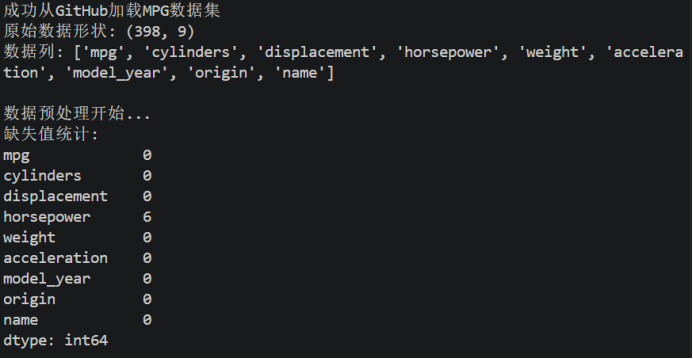
图5 MPG数据集结果展示
成功加载MPG数据集,列出9种数据列,且horsepower缺失6个。
2)代码运行结果
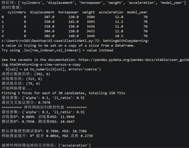
图6 独热编码法
模型仅使用数值型特征(气缸数、排量、马力、重量、加速度、年份),最佳参数:alpha=0.1、l1_ratio=0.9,测试集R²=0.7950,MSE=10.4647。弹性网络筛选掉的无关特征:acceleration(加速度),模型表现良好。
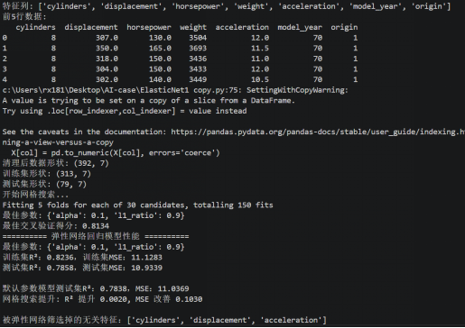
图7 数值映射法
在原有特征基础上增加了制造商地区(origin),并直接赋予数值 1、2、3。测试集R²=0.7858,MSE=10.9339,性能反而下降。筛选掉的无关特征增多:cylinders,displacement,acceleration。原因:origin是无序类别变量(如美国、欧洲、日本),直接映射为 1、2、3会引入虚假的顺序关系,误导模型,导致预测能力下降。
3)多维度可视化分析
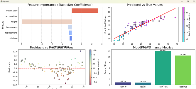
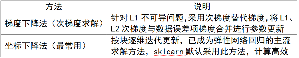
图8 特征重要性、测试集真实值vs预测值散点图、残差分布、模型性能指标对比
1 特征重要性:weight(重量)和 model_year(年份)的系数绝对值最大,表明它们是预测油耗最关键的变量;acceleration(加速度)的系数压缩为0,被筛选掉。可以理解为使用更轻、马力更小、排量小、气缸量小、年份更新的车辆通常具有更高的燃油效率。
2 预测值vs真实值:散点基本围绕对角线分布,但存在一定离散,表明模型预测能力中等。
3 残差vs预测值:残差点在零线附近随机分布,无明显漏斗形或趋势,说明模型满足线性回归的方差齐性假设,稳定性较好。
4 性能指标:训练集R²约0.810,测试集R²约0.795,训练MSE约11.99,测试MSE约10.46,说明模型未出现严重过拟合,泛化能力良好。
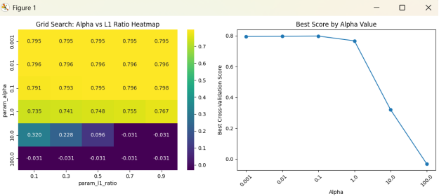
图9 网格搜索热力图和最佳得分随Alpha变化折线图
网格搜索热力图:
1 当alpha很小时(0.001-0.1),得分较高(约0.80-0.82),且对不同l1_ratio不敏感。
2 当alpha=1时,得分开始下降。
3 当alpha=10或100时,得分急剧下降到接近0或负数,说明正则化过强,模型欠拟合。
4 最佳参数通常出现在alpha=0.1或0.01,l1_ratio=0.9。
最佳分数与Alpha:
1 曲线在alpha较小时保持平稳高位。
2 在alpha=1处开始下降,alpha=10之后急剧下滑。
该图表明模型对正则化强度敏感,不宜使用过大的alpha。
4.问题分析
1)数值映射vs独热编码
1数值映射
优点:不增加特征维度,保持原特征数量。
缺点:引入虚假顺序关系(如usa=1,europe=2,japan=3),暗示类别间存在大小等级,与实际无序类别矛盾。
2 独热编码
优点:每个类别独立为一个二值特征,消除虚假顺序,真实表达平等类别关系。
配合L1正则化可自动对冗余虚拟变量进行特征选择。
本数据集实践:对origin(美国、欧洲、日本)采用独热编码,正确表达了三个地区的平等属性。
2)固定参数训练vs超参数优化策略
1 固定参数训练
直接使用默认或经验参数,缺乏合理性验证。
无法保证找到最优超参数,易导致次优性能。
2 网格搜索(GridSearchCV)
自动遍历指定超参数组合,结合交叉验证评估性能。
先通过交叉验证确定最佳参数,再训练最终模型,确保参数选择科学可靠。
后续使用更高效的搜索策略,在更大参数空间内快速找到全局最优解。