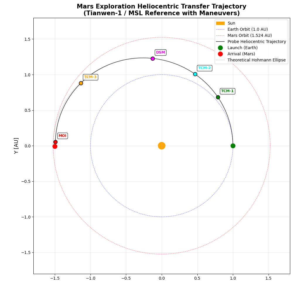
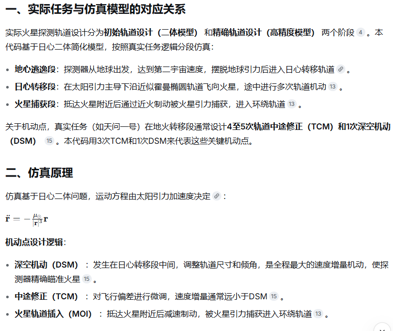
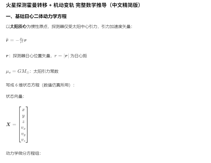
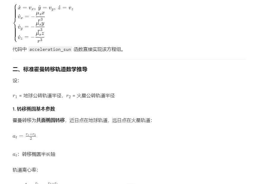
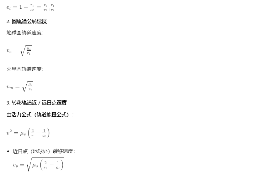
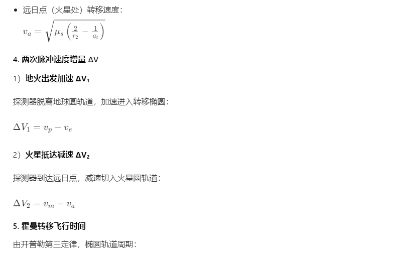
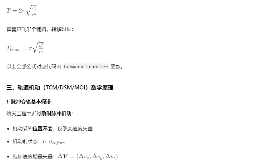
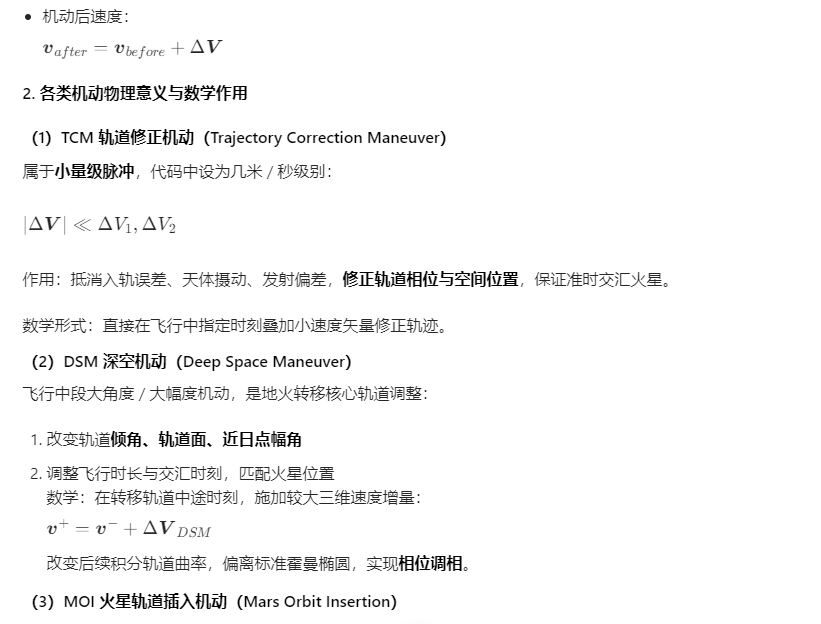
本文介绍了一个火星探测任务的轨道模拟程序,使用Python数值计算库模拟了从地球到火星的转移轨道。程序基于二体问题计算太阳引力作用下的航天器轨迹,采用Hohmann转移轨道理论设计初始轨道参数,并加入了五次轨道机动(包括深空机动和轨迹修正)。模拟结果显示:转移轨道半长轴1.262AU,偏心率0.207,总飞行时间202天,总ΔV预算约323.2m/s。程序输出了2D和3D可视化结果,展示了航天器从地球轨道出发,经多次机动后到达火星轨道的完整轨迹。该模拟为火星探测任务提供了轨道设计和机动规划的参考框架。
五、轨迹出现直线 / 错位问题的数学原因(原代码 bug 根源)
- 原积分未均匀布点
t_eval,仅用自适应步长,分段拼接时时间点稀疏,视觉出现直线段; - 机动状态赋值顺序错误,先存轨迹再改速度,造成轨迹点与机动不同步,重复画线;
- 修正方案:每段积分均匀取时间采样点,先积分结束再统一更新速度状态,保证轨迹连续光滑。
python
import numpy as np
from scipy.integrate import solve_ivp
import matplotlib.pyplot as plt
from matplotlib.patches import Circle
from mpl_toolkits.mplot3d import Axes3D

# ==================== Celestial Constants & Orbital Parameters ====================
# Astronomical Unit (AU) and time units (seconds)
AU = 1.495978707e11          # 1 AU [m]
DAY = 86400.0                # 1 day [s]
SIDEREAL_YEAR = 365.256363004 * DAY  # 1 sidereal year [s]

# Gravitational parameters
MU_SUN = 1.32712440018e20    # Sun gravitational parameter [m^3/s^2]
MU_EARTH = 3.986004418e14    # Earth gravitational parameter [m^3/s^2]
MU_MARS  = 4.282837e13       # Mars gravitational parameter [m^3/s^2]

# Sun radius (for visualization)
R_SUN = 6.957e8              # Sun radius [m]

# ==================== Mission Parameters ====================
T_FLIGHT = 202.0 * DAY       # Total flight time [s]

# ==================== Orbital Mechanics Helper Functions ====================
def norm(v):
    """Compute Euclidean norm of a vector"""
    return np.sqrt(np.dot(v, v))

def acceleration_sun(t, state):
    """
    Heliocentric two-body acceleration
    state: [x, y, z, vx, vy, vz]
    return: [vx, vy, vz, ax, ay, az]
    """
    r_vec = state[:3]
    r = norm(r_vec)
    a_grav = -MU_SUN / r**3 * r_vec
    return np.concatenate([state[3:], a_grav])

def hohmann_transfer(r1, r2):
    """
    Calculate Hohmann transfer orbit parameters
    r1: Earth orbit radius [m] (circular approximation)
    r2: Mars orbit radius [m] (circular approximation)
    return: semi-major axis, velocity increments, transfer time, velocities
    """
    a_trans = (r1 + r2) / 2.0
    v_earth = np.sqrt(MU_SUN / r1)
    v_perihelion = np.sqrt(2*MU_SUN/r1 - MU_SUN/a_trans)
    v_aphelion = np.sqrt(2*MU_SUN/r2 - MU_SUN/a_trans)
    v_mars = np.sqrt(MU_SUN / r2)
    delta_v1 = v_perihelion - v_earth
    delta_v2 = v_mars - v_aphelion
    T_trans = np.pi * np.sqrt(a_trans**3 / MU_SUN)
    return a_trans, delta_v1, delta_v2, T_trans, v_perihelion, v_aphelion

# ==================== Main Simulation ====================
def simulate_mars_mission():
    """
    Mars exploration mission trajectory simulation
    Includes: heliocentric transfer with deep space maneuver and trajectory corrections
    """
    # Simplified circular orbit parameters
    r_earth = 1.0 * AU
    r_mars  = 1.524 * AU

    # Hohmann transfer calculation
    a_trans, dv1, dv2, T_trans, v_perihelion, v_aphelion = hohmann_transfer(r_earth, r_mars)
    e_trans = 1.0 - r_earth / a_trans

    print("="*60)
    print("MARS EXPLORATION ORBIT SIMULATION PARAMETERS")
    print("="*60)
    print(f"Transfer semi-major axis:      {a_trans/AU:.4f} AU")
    print(f"Transfer eccentricity:         {e_trans:.4f}")
    print(f"Hohmann transfer time:         {T_trans/DAY:.2f} days")
    print(f"ΔV1 (Departure burn):          {dv1:.2f} m/s")
    print(f"ΔV2 (Arrival burn):            {dv2:.2f} m/s")
    print(f"Perihelion velocity:           {v_perihelion:.2f} m/s")
    print(f"Aphelion velocity:             {v_aphelion:.2f} m/s")
    print(f"Total flight time:             {T_FLIGHT/DAY:.2f} days")
    print("="*60)

    # Maneuver timeline
    t_dsm  = 0.40 * T_trans
    t_tcm1 = 0.15 * T_trans
    t_tcm2 = 0.25 * T_trans
    t_tcm3 = 0.70 * T_trans
    t_moi  = 0.98 * T_trans

    maneuvers = {
        "TCM-1": {"t": t_tcm1, "dv": np.array([15.0, 0.0, 0.0])},
        "TCM-2": {"t": t_tcm2, "dv": np.array([0.0, 10.0, 0.0])},
        "DSM":   {"t": t_dsm,  "dv": np.array([250.0, 0.0, -50.0])},
        "TCM-3": {"t": t_tcm3, "dv": np.array([8.0, 0.0, 0.0])},
        "MOI":   {"t": t_moi,  "dv": np.array([-dv2, 0.0, 0.0])},
    }

    print("\nManeuver Timeline:")
    print("-"*60)
    for name, m in maneuvers.items():
        print(f"  {name:6s}: t = {m['t']/DAY:8.2f} days, |ΔV| = {norm(m['dv']):8.2f} m/s")
    print("="*60)

    # Initial state
    v_earth = np.sqrt(MU_SUN / r_earth)
    r0 = np.array([r_earth, 0.0, 0.0])
    v0 = np.array([0.0, v_earth + dv1, 0.0])
    state0 = np.concatenate([r0, v0])

    print(f"\nInitial State:")
    print(f"  Position: [{r0[0]/AU:.4f}, {r0[1]/AU:.4f}, {r0[2]/AU:.4f}] AU")
    print(f"  Velocity: [{v0[0]:.2f}, {v0[1]:.2f}, {v0[2]:.2f}] m/s")
    print(f"  Departure ΔV: {dv1:.2f} m/s")

    # Segmented integration with smooth time points
    t_events = sorted([m["t"] for m in maneuvers.values()])
    t_events = [0.0] + t_events + [T_trans]

    trajectory_segments = []
    time_segments = []
    maneuver_points = []
    current_state = state0.copy()

    for i in range(len(t_events) - 1):
        t_start = t_events[i]
        t_end   = t_events[i + 1]

        # Generate smooth time points for continuous curve
        t_eval = np.linspace(t_start, t_end, 100)

        # Integrate trajectory segment
        sol = solve_ivp(
            acceleration_sun,
            [t_start, t_end],
            current_state,
            method='DOP853',
            t_eval=t_eval,
            rtol=1e-10,
            atol=1e-10
        )

        # Store segment data
        trajectory_segments.append(sol.y.T)
        time_segments.append(sol.t)

        # Update state and apply maneuver
        current_state = sol.y[:, -1].copy()

        if t_end < T_trans:
            for name, m in maneuvers.items():
                if abs(m["t"] - t_end) < 1.0:
                    r_pre = current_state[:3].copy()
                    v_pre = current_state[3:].copy()

                    maneuver_points.append({
                        "name": name,
                        "t": t_end,
                        "r": r_pre.copy(),
                        "v_before": v_pre.copy(),
                        "dv": m["dv"].copy(),
                        "v_after": v_pre + m["dv"]
                    })

                    print(f"\n>>> Maneuver [{name}] @ t = {t_end/DAY:.2f} days")
                    print(f"    Position: [{r_pre[0]/AU:.4f}, {r_pre[1]/AU:.4f}, {r_pre[2]/AU:.4f}] AU")
                    print(f"    Velocity before: [{v_pre[0]:.2f}, {v_pre[1]:.2f}, {v_pre[2]:.2f}] m/s")
                    print(f"    ΔV: [{m['dv'][0]:.2f}, {m['dv'][1]:.2f}, {m['dv'][2]:.2f}] m/s")
                    print(f"    |ΔV| = {norm(m['dv']):.2f} m/s")

                    current_state[3:] = v_pre + m["dv"]
                    break

    # Combine all segments
    trajectory = np.vstack(trajectory_segments)
    time_array = np.hstack(time_segments)

    return trajectory, time_array, maneuver_points, r_earth, r_mars, T_trans

# ==================== Main Execution ====================
if __name__ == "__main__":
    # Run simulation
    trajectory, time_array, maneuver_points, r_earth, r_mars, T_trans = simulate_mars_mission()

    # ==================== 2D Heliocentric Trajectory Visualization ====================
    fig, ax = plt.subplots(1, 1, figsize=(12, 10))

    # Plot Sun
    sun = Circle((0, 0), 0.05, color='orange', label='Sun')
    ax.add_patch(sun)

    # Plot orbits
    theta = np.linspace(0, 2*np.pi, 360)
    earth_orbit_x = r_earth / AU * np.cos(theta)
    earth_orbit_y = r_earth / AU * np.sin(theta)
    ax.plot(earth_orbit_x, earth_orbit_y, 'b--', linewidth=0.8, alpha=0.5, label='Earth Orbit (1.0 AU)')

    mars_orbit_x = r_mars / AU * np.cos(theta)
    mars_orbit_y = r_mars / AU * np.sin(theta)
    ax.plot(mars_orbit_x, mars_orbit_y, 'r--', linewidth=0.8, alpha=0.5, label='Mars Orbit (1.524 AU)')

    # Plot smooth probe trajectory
    traj_x = trajectory[:, 0] / AU
    traj_y = trajectory[:, 1] / AU
    ax.plot(traj_x, traj_y, 'k-', linewidth=1.2, alpha=0.8, label='Probe Heliocentric Trajectory')

    # Plot maneuver points
    colors = {'TCM-1': 'green', 'TCM-2': 'cyan', 'DSM': 'magenta', 'TCM-3': 'orange', 'MOI': 'red'}
    for mp in maneuver_points:
        c = colors.get(mp["name"], 'blue')
        ax.plot(mp["r"][0]/AU, mp["r"][1]/AU, 'o', color=c, markersize=9,
                markeredgecolor='black', markeredgewidth=1.2, zorder=5)
        ax.annotate(mp["name"],
                    (mp["r"][0]/AU, mp["r"][1]/AU),
                    xytext=(8, 12), textcoords='offset points',
                    fontsize=9, fontweight='bold', color=c,
                    bbox=dict(boxstyle='round,pad=0.3', facecolor='white', alpha=0.8))

    # Plot launch and arrival points
    ax.plot(traj_x[0], traj_y[0], 'go', markersize=11, label='Launch (Earth)')
    ax.plot(traj_x[-1], traj_y[-1], 'ro', markersize=11, label='Arrival (Mars)')

    # Plot theoretical Hohmann ellipse
    a_trans_au = (r_earth + r_mars) / (2 * AU)
    c_au = (r_mars - r_earth) / (2 * AU)
    b_au = np.sqrt(a_trans_au**2 - c_au**2)
    center_x = -c_au
    ellipse_theta = np.linspace(0, np.pi, 200)
    ellipse_x = center_x + a_trans_au * np.cos(ellipse_theta)
    ellipse_y = b_au * np.sin(ellipse_theta)
    ax.plot(ellipse_x, ellipse_y, 'gray', linewidth=1.2, linestyle=':', alpha=0.6, label='Theoretical Hohmann Ellipse')

    # Plot settings
    ax.set_xlabel('X [AU]', fontsize=13)
    ax.set_ylabel('Y [AU]', fontsize=13)
    ax.set_title('Mars Exploration Heliocentric Transfer Trajectory\n(Tianwen-1 / MSL Reference with Maneuvers)',
                 fontsize=15, fontweight='bold')
    ax.legend(loc='upper right', fontsize=10)
    ax.set_aspect('equal')
    ax.grid(True, alpha=0.3)
    ax.set_xlim(-1.8, 1.8)
    ax.set_ylim(-1.8, 1.8)

    plt.tight_layout()
    plt.savefig('mars_mission_trajectory_2d.png', dpi=150)
    plt.show()

    # ==================== 3D Trajectory Visualization ====================
    fig3d = plt.figure(figsize=(14, 10))
    ax3d = fig3d.add_subplot(111, projection='3d')

    # 3D trajectory
    ax3d.plot(trajectory[:, 0]/AU, trajectory[:, 1]/AU, trajectory[:, 2]/AU,
              'k-', linewidth=1.2, alpha=0.8, label='Probe Trajectory')

    # 3D orbits
    ax3d.plot(earth_orbit_x, earth_orbit_y, np.zeros_like(earth_orbit_x),
              'b--', linewidth=0.8, alpha=0.5, label='Earth Orbit')
    ax3d.plot(mars_orbit_x, mars_orbit_y, np.zeros_like(mars_orbit_x),
              'r--', linewidth=0.8, alpha=0.5, label='Mars Orbit')

    # 3D maneuver points
    for mp in maneuver_points:
        c = colors.get(mp["name"], 'blue')
        ax3d.scatter(mp["r"][0]/AU, mp["r"][1]/AU, mp["r"][2]/AU,
                    color=c, s=90, edgecolors='black', linewidth=1.2, zorder=5)
        ax3d.text(mp["r"][0]/AU, mp["r"][1]/AU, mp["r"][2]/AU,
                 f'  {mp["name"]}', fontsize=9, fontweight='bold', color=c)

    # Sun
    ax3d.scatter(0, 0, 0, color='orange', s=300, label='Sun')

    # 3D plot settings
    ax3d.set_xlabel('X [AU]', fontsize=12)
    ax3d.set_ylabel('Y [AU]', fontsize=12)
    ax3d.set_zlabel('Z [AU]', fontsize=12)
    ax3d.set_title('Mars Exploration Heliocentric Transfer Trajectory (3D View)',
                   fontsize=14, fontweight='bold')
    ax3d.legend(loc='upper right', fontsize=9)

    max_range = 2.0
    ax3d.set_xlim(-max_range, max_range)
    ax3d.set_ylim(-max_range, max_range)
    ax3d.set_zlim(-0.5, 0.5)

    plt.tight_layout()
    plt.savefig('mars_mission_trajectory_3d.png', dpi=150)
    plt.show()

    # ==================== Simulation Summary ====================
    print("\n" + "="*60)
    print("SIMULATION SUMMARY")
    print("="*60)
    print(f"Total data points: {len(trajectory)}")
    print(f"Flight duration: {T_trans/DAY:.2f} days (~{T_trans/DAY/30.44:.1f} months)")
    print(f"Total maneuvers: {len(maneuver_points)}")
    total_dv = sum([norm(mp['dv']) for mp in maneuver_points])
    print(f"Total ΔV budget: {total_dv:.2f} m/s")

    print("\nManeuver Details:")
    for mp in maneuver_points:
        print(f"  {mp['name']:6s} | t={mp['t']/DAY:7.2f}d | |ΔV|={norm(mp['dv']):8.2f} m/s | "
              f"r=({mp['r'][0]/AU:.3f}, {mp['r'][1]/AU:.3f}, {mp['r'][2]/AU:.3f}) AU")
    print("="*60)