案例:信用卡欺诈分类
案例背景
数据集包含2013年9月欧洲持卡人的信用卡交易。
该数据集显示了两天内发生的交易,其中284,807宗交易中只有492个欺诈。
数据集高度不平衡,正类(欺诈交易)仅占所有交易的0.172%。
它只包含数值输入变量,这是一个PCA变换的结果。
出于保密问题,没有提供原始特征和更多关于数据的背景信息。
特征V1, V2,...V28为主成分分析(PCA)得到的主成分;
唯一没有使用PCA转换的特征是时间和数量。
Feature Time包含每个事务与数据集中的第一个事务之间所经过的秒数。
特征Amount是指交易金额,此特征可用于示例依赖的成本敏感学习。
Feature Class是标签变量,如果发生欺诈,它的值为1,否则为0。
数据读取与划分
python
import pandas as pd
import numpy as np
import matplotlib
from IPython.display import Image
import matplotlib.pyplot as plt
import seaborn as sns
%matplotlib inline
import plotly.graph_objs as go
import plotly.figure_factory as ff
from plotly import tools
from plotly.offline import download_plotlyjs, init_notebook_mode, plot, iplot
init_notebook_mode(connected=True)

import warnings
warnings.filterwarnings('ignore')

import gc
from sklearn.model_selection import train_test_split
from sklearn.metrics import accuracy_score , f1_score ,roc_auc_score
from sklearn.ensemble import AdaBoostClassifier,GradientBoostingClassifier
from xgboost import XGBClassifier

pd.set_option('display.max_columns', 100)

#TRAIN/TEST SPLIT
TEST_SIZE = 0.20 # test size using_train_test_split

RANDOM_STATE = 42
接着读取数据,并且输出数据的信息
python
data = pd.read_csv("./creditcard.csv")

print("Credit Card Fraud Detection data - rows:",data.shape[0]," columns:", data.shape[1])Credit Card Fraud Detection data - rows: 284807 columns: 31接着使用head观察数据
python
data.head()| | Time | V1 | V2 | V3 | V4 | V5 | V6 | V7 | V8 | V9 | V10 | V11 | V12 | V13 | V14 | V15 | V16 | V17 | V18 | V19 | V20 | V21 | V22 | V23 | V24 | V25 | V26 | V27 | V28 | Amount | Class |
| 0 | 0.0 | -1.359807 | -0.072781 | 2.536347 | 1.378155 | -0.338321 | 0.462388 | 0.239599 | 0.098698 | 0.363787 | 0.090794 | -0.551600 | -0.617801 | -0.991390 | -0.311169 | 1.468177 | -0.470401 | 0.207971 | 0.025791 | 0.403993 | 0.251412 | -0.018307 | 0.277838 | -0.110474 | 0.066928 | 0.128539 | -0.189115 | 0.133558 | -0.021053 | 149.62 | 0 |
| 1 | 0.0 | 1.191857 | 0.266151 | 0.166480 | 0.448154 | 0.060018 | -0.082361 | -0.078803 | 0.085102 | -0.255425 | -0.166974 | 1.612727 | 1.065235 | 0.489095 | -0.143772 | 0.635558 | 0.463917 | -0.114805 | -0.183361 | -0.145783 | -0.069083 | -0.225775 | -0.638672 | 0.101288 | -0.339846 | 0.167170 | 0.125895 | -0.008983 | 0.014724 | 2.69 | 0 |
| 2 | 1.0 | -1.358354 | -1.340163 | 1.773209 | 0.379780 | -0.503198 | 1.800499 | 0.791461 | 0.247676 | -1.514654 | 0.207643 | 0.624501 | 0.066084 | 0.717293 | -0.165946 | 2.345865 | -2.890083 | 1.109969 | -0.121359 | -2.261857 | 0.524980 | 0.247998 | 0.771679 | 0.909412 | -0.689281 | -0.327642 | -0.139097 | -0.055353 | -0.059752 | 378.66 | 0 |
| 3 | 1.0 | -0.966272 | -0.185226 | 1.792993 | -0.863291 | -0.010309 | 1.247203 | 0.237609 | 0.377436 | -1.387024 | -0.054952 | -0.226487 | 0.178228 | 0.507757 | -0.287924 | -0.631418 | -1.059647 | -0.684093 | 1.965775 | -1.232622 | -0.208038 | -0.108300 | 0.005274 | -0.190321 | -1.175575 | 0.647376 | -0.221929 | 0.062723 | 0.061458 | 123.50 | 0 |
| 4 | 2.0 | -1.158233 | 0.877737 | 1.548718 | 0.403034 | -0.407193 | 0.095921 | 0.592941 | -0.270533 | 0.817739 | 0.753074 | -0.822843 | 0.538196 | 1.345852 | -1.119670 | 0.175121 | -0.451449 | -0.237033 | -0.038195 | 0.803487 | 0.408542 | -0.009431 | 0.798278 | -0.137458 | 0.141267 | -0.206010 | 0.502292 | 0.219422 | 0.215153 | 69.99 | 0 |
|---|
从数据结果中看到数据集中共284,807条记录
查看数据集中的数据缺失情况
python
total = data.isnull().sum().sort_values(ascending = False)
percent = (data.isnull().sum()/data.isnull().count()*100).sort_values(ascending = False)
pd.concat([total, percent], axis=1, keys=['Total', 'Percent']).transpose()
| | Time | V16 | Amount | V28 | V27 | V26 | V25 | V24 | V23 | V22 | V21 | V20 | V19 | V18 | V17 | V15 | V1 | V14 | V13 | V12 | V11 | V10 | V9 | V8 | V7 | V6 | V5 | V4 | V3 | V2 | Class |
| Total | 0.0 | 0.0 | 0.0 | 0.0 | 0.0 | 0.0 | 0.0 | 0.0 | 0.0 | 0.0 | 0.0 | 0.0 | 0.0 | 0.0 | 0.0 | 0.0 | 0.0 | 0.0 | 0.0 | 0.0 | 0.0 | 0.0 | 0.0 | 0.0 | 0.0 | 0.0 | 0.0 | 0.0 | 0.0 | 0.0 | 0.0 |
| Percent | 0.0 | 0.0 | 0.0 | 0.0 | 0.0 | 0.0 | 0.0 | 0.0 | 0.0 | 0.0 | 0.0 | 0.0 | 0.0 | 0.0 | 0.0 | 0.0 | 0.0 | 0.0 | 0.0 | 0.0 | 0.0 | 0.0 | 0.0 | 0.0 | 0.0 | 0.0 | 0.0 | 0.0 | 0.0 | 0.0 | 0.0 |
|---|
从上面的结果来看,数据集中不存在缺失数据
按照是否被欺诈进行分类可视化
python
temp = data["Class"].value_counts()
df = pd.DataFrame({'Class': temp.index,'values': temp.values})

trace = go.Bar(
    x = df['Class'],y = df['values'],
    name="Credit Card Fraud Class - data unbalance (Not fraud = 0, Fraud = 1)",
    marker=dict(color="Blue"),
    text=df['values']
)
temp_data = [trace]
layout = dict(title = 'Credit Card Fraud Class - data unbalance (Not fraud = 0, Fraud = 1)',
          xaxis = dict(title = 'Class', showticklabels=True),
          yaxis = dict(title = 'Number of transactions'),
          hovermode = 'closest',width=600
         )
fig = dict(data=temp_data, layout=layout)
iplot(fig, filename='class')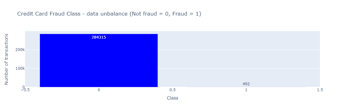
从可视化结果来看,数据集中是存在数据不平衡性的,只有492条诈骗记录(0.172%)
接下来对欺诈案例按照时间维度进行可视化
python
class_0 = data.loc[data['Class'] == 0]["Time"]
class_1 = data.loc[data['Class'] == 1]["Time"]

hist_data = [class_0, class_1]
group_labels = ['Not Fraud', 'Fraud']

fig = ff.create_distplot(hist_data, group_labels, show_hist=False, show_rug=False)
fig['layout'].update(title='Credit Card Transactions Time Density Plot', xaxis=dict(title='Time [s]'))
iplot(fig, filename='dist_only')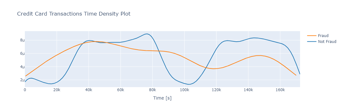
从结果来看,欺诈交易分布的较为均匀,且容易在夜间持续发生。
接下来将将数据分为训练集和测试集
python
train_df, test_df = train_test_split(data, test_size=TEST_SIZE, random_state=RANDOM_STATE, shuffle=True)由于数据集中存在数据不平衡的现象,因此需要对训练数据进行平衡,通过对数量较多的非欺诈样本进行欠采样,将欺诈样本的比例提升到1%
python
# 获得欺诈样本的数量
train_fraud_df  = train_df[train_df['Class'] ==1]
no_of_fraud = train_fraud_df.shape[0]

# 对非欺诈样本进行欠采样
no_of_non_fraud = no_of_fraud * 99
train_non_fraud_df = train_df[train_df['Class'] ==0].sample( no_of_non_fraud , random_state =RANDOM_STATE)
no_of_non_fraud = train_non_fraud_df.shape[0]

# 将欠采样后的数据进行整合,并且对数据的顺序进行打乱

train_df = pd.concat([train_fraud_df, train_non_fraud_df] , axis =0 )
train_df = train_df.sample(frac = 1,random_state =RANDOM_STATE)Total Fraud in Train Data : 394
Total non Fraud in Train Data : 39006
python
target = 'Class'
predictors = ['Time', 'V1', 'V2', 'V3', 'V4', 'V5', 'V6', 'V7', 'V8', 'V9', 'V10',\
       'V11', 'V12', 'V13', 'V14', 'V15', 'V16', 'V17', 'V18', 'V19',\
       'V20', 'V21', 'V22', 'V23', 'V24', 'V25', 'V26', 'V27', 'V28',\
       'Amount']
AdaBoost模型搭建与训练
python
ada_clf = AdaBoostClassifier(random_state=RANDOM_STATE)

ada_clf.fit(train_df[predictors], train_df[target].values)

test_df['prediction'] = ada_clf.predict(test_df[predictors])

cm = pd.crosstab(test_df[target].values, test_df['prediction'], rownames=['Actual'], colnames=['Predicted'])
fig, ax1 = plt.subplots(ncols=1, figsize=(7,7))
sns.heatmap(cm,
            xticklabels=['Not Fraud', 'Fraud'],
            yticklabels=['Not Fraud', 'Fraud'],
            annot=True,ax=ax1,
            linewidths=.2,linecolor="Darkblue", cmap="Blues" , fmt='d')
plt.title('Confusion Matrix', fontsize=16)
plt.show()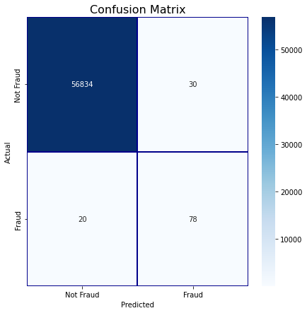
python
metric_data = pd.DataFrame(columns =['Model Name','Detection Rate' ,'AUC','F1 Score','Accuracy','Fraud Loss Saved'])
python
# we will use original data as Amount is transformed for modelling
def fraud_loss_saved ( dataset , key) :

    df = dataset.copy()
    total_fraud_amt = df[df['Class'] ==1]['Amount'].sum()
    print("Total Fraud Amount in Test Data : " +  str(round(total_fraud_amt,2)))
    total_fraud_amt_detected = df.loc[(df['prediction'] ==1) & (df['Class']==1) ]['Amount'].sum()
    print("Total Fraud Amount Detected in Test Data : " +  str(round(total_fraud_amt_detected,2)))
    print("Fraud Loss Saved (%): " + str(round(100*total_fraud_amt_detected/total_fraud_amt ,2)))
    detection_rate  = 100 * (df[df['prediction']==1]['Class'].sum())/df['Class'].sum()
    print("Detection Rate (%) : " + str(round(detection_rate , 2)))
    accuracy = 100*accuracy_score(df['Class'] ,df['prediction'])
    print("Accuracy : " + str(round(accuracy ,2)))
    f1 = f1_score(df['Class'] ,df['prediction'])
    print("F1 Score : " + str(round(f1 ,4)))
    auc_score = roc_auc_score(df['Class'],df['prediction'])
    print("AUC Score : " + str(round(auc_score,4)))
    values = []
    values.append(key)
    values.append(detection_rate)
    values.append(auc_score)
    values.append(f1)
    values.append(accuracy)
    values.append(round(100*total_fraud_amt_detected/total_fraud_amt ,2))

    final_values =[]
    final_values.append(values)
    temp_df = pd.DataFrame(final_values ,columns =['Model Name','Detection Rate' ,'AUC','F1 Score','Accuracy','Fraud Loss Saved'])

    global metric_data

    metric_data = pd.concat([metric_data,temp_df ] , axis = 0 )
python
fraud_loss_saved(test_df ,'AdaBoost - Test Data')Total Fraud Amount in Test Data : 16078.4
Total Fraud Amount Detected in Test Data : 12019.13
Fraud Loss Saved (%): 74.75
Detection Rate (%) : 79.59
Accuracy : 99.91
F1 Score : 0.7573
AUC Score : 0.8977GBDT模型搭建与训练
python
gbdf_clf = GradientBoostingClassifier(random_state=RANDOM_STATE)

gbdf_clf.fit(train_df[predictors], train_df[target].values)

test_df['prediction'] = gbdf_clf.predict(test_df[predictors])

cm = pd.crosstab(test_df[target].values, test_df['prediction'], rownames=['Actual'], colnames=['Predicted'])
fig, ax1 = plt.subplots(ncols=1, figsize=(7,7))
sns.heatmap(cm,
            xticklabels=['Not Fraud', 'Fraud'],
            yticklabels=['Not Fraud', 'Fraud'],
            annot=True,ax=ax1,
            linewidths=.2,linecolor="Darkblue", cmap="Blues" , fmt='d')
plt.title('Confusion Matrix', fontsize=16)
plt.show()
python
fraud_loss_saved(test_df ,'GBDT - Test Data')Total Fraud Amount in Test Data : 16078.4
Total Fraud Amount Detected in Test Data : 12252.02
Fraud Loss Saved (%): 76.2
Detection Rate (%) : 82.65
Accuracy : 99.79
F1 Score : 0.5724
AUC Score : 0.9124XGBoost模型搭建与训练
python
xgb_clf = XGBClassifier(random_state=RANDOM_STATE)

xgb_clf.fit(train_df[predictors], train_df[target].values)

test_df['prediction'] = xgb_clf.predict(test_df[predictors])

cm = pd.crosstab(test_df[target].values, test_df['prediction'], rownames=['Actual'], colnames=['Predicted'])
fig, ax1 = plt.subplots(ncols=1, figsize=(7,7))
sns.heatmap(cm,
            xticklabels=['Not Fraud', 'Fraud'],
            yticklabels=['Not Fraud', 'Fraud'],
            annot=True,ax=ax1,
            linewidths=.2,linecolor="Darkblue", cmap="Blues" , fmt='d')
plt.show()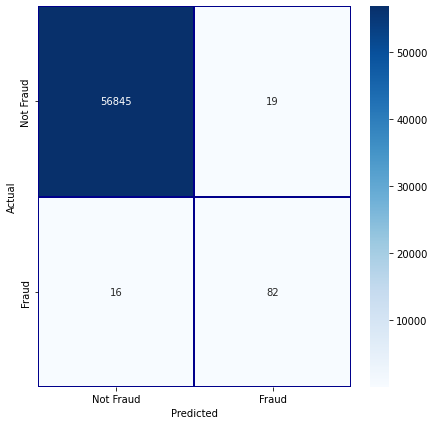
python
fraud_loss_saved(test_df ,'XGBoost - Test Data')Total Fraud Amount in Test Data : 16078.4
Total Fraud Amount Detected in Test Data : 12346.92
Fraud Loss Saved (%): 76.79
Detection Rate (%) : 83.67
Accuracy : 99.94
F1 Score : 0.8241
AUC Score : 0.9182模型对比
python
metric_data| | Model Name | Detection Rate | AUC | F1 Score | Accuracy | Fraud Loss Saved |
| 0 | AdaBoost - Test Data | 79.591837 | 0.897695 | 0.757282 | 99.912222 | 74.75 |
| 0 | GBDT - Test Data | 82.653061 | 0.912351 | 0.572438 | 99.787578 | 76.20 |
| 0 | XGBoost - Test Data | 83.673469 | 0.918200 | 0.824121 | 99.938556 | 76.79 |
|---|
从结果中可以看到,在3个模型当中,XGBoost模型具有最好的效果,能够帮助更加准确的识别出欺诈行为,进而帮助我们保护更多的财产。