笔记：TREX工具-1

TensorRT Engine Explorer (trex) 使用指南

概述

trex 是基于 TensorRT 导出 JSON 文件的分析工具。

工作流程：

复制代码

ONNX模型 → trtexec 构建引擎 → 导出 JSON → trex 分析引擎

核心文件

trex 分析依赖三个 JSON 文件：

文件	内容	生成方式
`.graph.json`	层的连接关系、类型、输入输出维度、权重信息	`trtexec --exportLayerInfo=<path>`
`.profile.json`	各层的执行时间、迭代次数、调用次数、显存占用等原始性能数据	`trtexec --exportProfile=<path>`
`.profile.metadata.json`	从日志解析的汇总信息（引擎延迟的 min/max/avg/median/p99、吞吐量 IPS、推理选项、设备信息等）	`parse_trtexec_log.py` 解析 trtexec 日志

数据来源说明：

分别 profiling 各层 → 提供每层延迟信息
整个引擎 profiling → 提供更准确的延迟和推理吞吐量值

关键指标解释：

平均时间：分别 profiling 各层时，层延迟的总和
延迟：引擎延迟测量的 $最小、最大、平均、中位数、99百分位$
吞吐量：每秒推理次数（IPS）

TensorRT 层类型

类型	功能
Convolution	卷积运算（卷积核滑动计算）
Pooling	池化操作（MaxPool / AvgPool）
Reformat	格式重排（FP32↔FP16/INT8、CHW↔HWC、GPU↔CPU）
MatrixMultiply	矩阵乘法（GEMM）
FullyConnected	全连接层（InnerProduct / Dense）
ElementWise	逐元素运算（Add / Mul / Sub / Div 等）
Activation	激活函数（ReLU / Sigmoid / Tanh 等）
SoftMax	Softmax 归一化指数函数
Reduce	降维操作（Sum / Max / Avg / Prod）
Concatenation	张量拼接
Slice	张量切片/截取
Reshape	张量形状变换
Shuffle	重排维度 + reshape
TopK	取最大/最小的 K 个值
Gather	索引收集张量元素
Identity	恒等变换（直接传递，不做计算）
Plugin	自定义插件层（用户扩展）
Scale	仿射变换（scale * x + shift）
Unary	一元运算（Exp / Log / Sin / Cos / Sqrt / Abs 等）
BatchNorm	批归一化（通常融合到 Conv 中）
Padding	填充操作
RNN	循环神经网络（LSTM / GRU）
QuantizeLinear	FP32 → INT8 量化
DequantizeLinear	INT8 → FP32 反量化
DetectionOutput	目标检测后处理（YOLO / SSD 等）
Normalize	L2 / L1 归一化
Split	张量分割成多个输出
Squeeze	移除维度为 1 的轴
Expand	广播扩展维度

Python API 使用

加载引擎

python 复制代码

import trex
import trex.notebook
import trex.plotting
import trex.graphing
import trex.df_preprocessing

# 配置宽屏显示
trex.notebook.set_wide_display()

# 加载引擎
engine_name = "../tests/inputs/mobilenet_v2_residuals.qat.onnx.engine"
plan = trex.EnginePlan(
    f'{engine_name}.graph.json',
    f'{engine_name}.profile.json',
    f'{engine_name}.profile.metadata.json'
)
print(f"Summary for {plan.name}:")
plan.summary()

查看数据

python 复制代码

# 查看 DataFrame 内容
trex.notebook.display_df(plan.df)

# 统计各层类型数量
layer_types = trex.group_count(plan.df, 'type')
trex.notebook.display_df(layer_types)

# 获取特定类型的所有层
convs = plan.get_layers_by_type('Convolution')
trex.notebook.display_df(convs)

输出示例

复制代码

Summary for mobilenet_v2_residuals.qat.onnx.engine.graph.json:
Model:
    Inputs: inputs.1: [1, 3, 224, 224]xFP32 NCHW
    Outputs: 1304: [1, 1000]xFP32 NCHW
    Average time: 0.356 ms
    Layers: 57
    Weights: 3.3 MB
    Activations: 14.2 MB
Device Properties:
    Selected Device: NVIDIA TITAN RTX
    Compute Capability: 7.5
    SMs: 72.0
    Compute Clock Rate: 1.77
    Device Global Memory: 24217 MiB
Performance Summary:
    Throughput: 3765.71
    Latency: [0.255981, 0.901474, 0.263917, 0.25824, 0.26123, 0.278473, 0.38501]

可视化分析

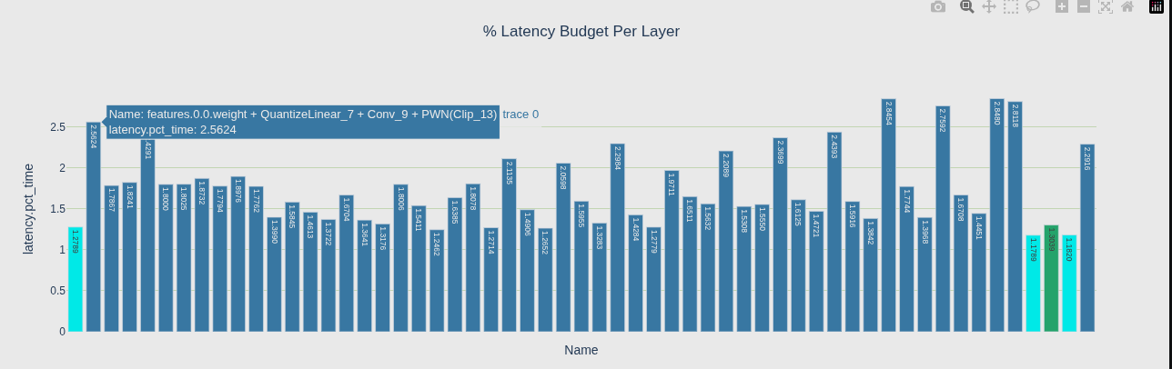
1. 层延迟视图

2. 层延迟树状矩形图

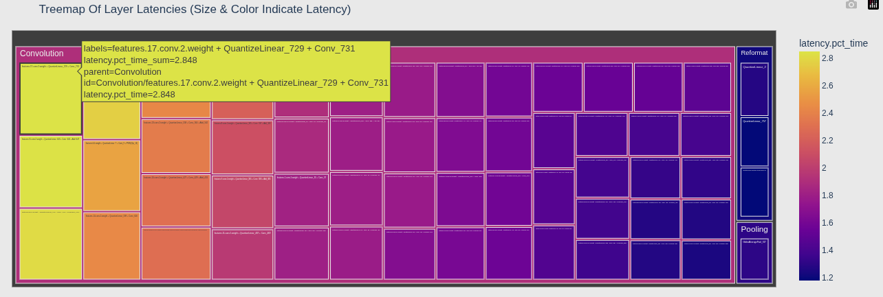
元素	含义
矩形大小	由 `values='latency.pct_time'` 决定 --- 矩形越大，该层占总延迟百分比越高
矩形颜色	由 `color='latency.pct_time'` 决定 --- 颜色越深/暖，延迟越高
层级结构	`path=['type', 'Name']` --- 外层是 type，内层是具体层名

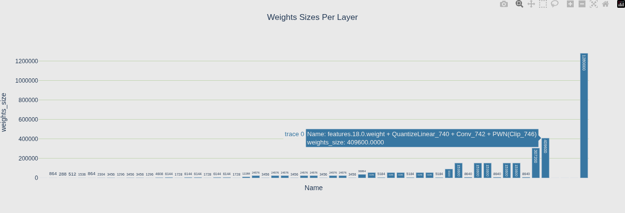
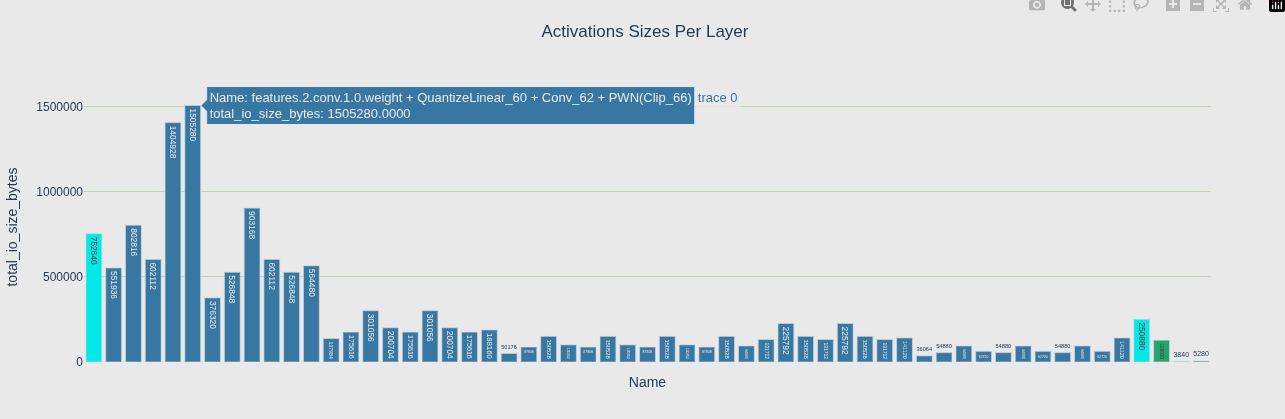
3. 内存分析

Weights 视图 - 静态权重谁最大（构建时就固定）

Activations 视图 - 动态中间结果谁最大（推理时临时分配）

Histogram 视图 - 整体分布，有没有离谱的 outlier

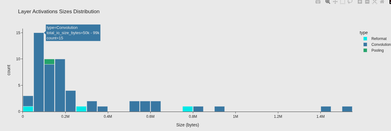
图	告诉你的问题
Weights	静态权重谁最大（构建时就固定）
Activations	动态中间结果谁最大（推理时临时分配）
Histogram	整体分布，有没有离谱的 outlier

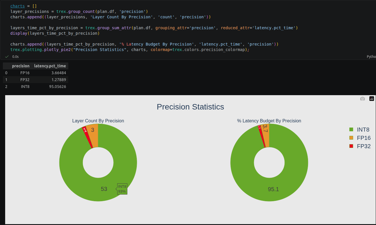
4. 层精度占比

展示各层使用的精度分布（FP32/FP16/INT8）。

5. 计算图可视化

python 复制代码

formatter = trex.graphing.layer_type_formatter if True else trex.graphing.precision_formatter
graph = trex.graphing.to_dot(plan, formatter)
svg_name = trex.graphing.render_dot(graph, engine_name, 'svg')

计算图的样子，类似netron

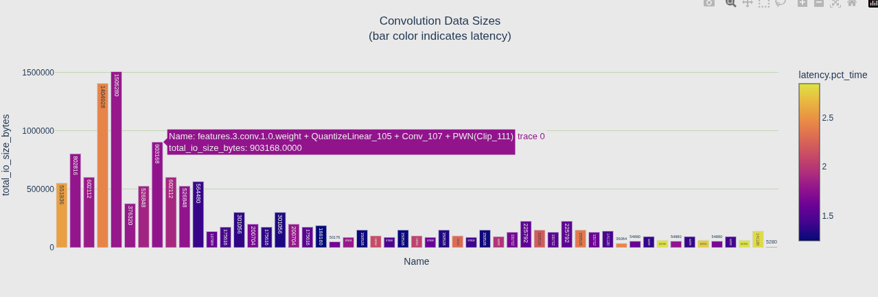
卷积层详细分析

python 复制代码

convs = plan.get_layers_by_type('Convolution')
trex.notebook.display_df(convs)

# 按精度着色的延迟图
trex.plotting.plotly_bar2(
    convs,
    "Latency Per Layer (%)<BR>(bar color indicates precision)",
    "attr.arithmetic_intensity", "Name",
    color='precision',
    colormap=trex.colors.precision_colormap)

# 按延迟着色的数据大小图
trex.plotting.plotly_bar2(
    convs,
    "Convolution Data Sizes<BR>(bar color indicates latency)",
    "total_io_size_bytes",
    "Name",
    color='latency.pct_time')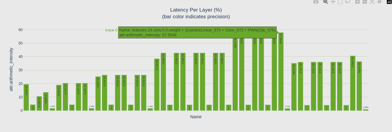

性能指标详解

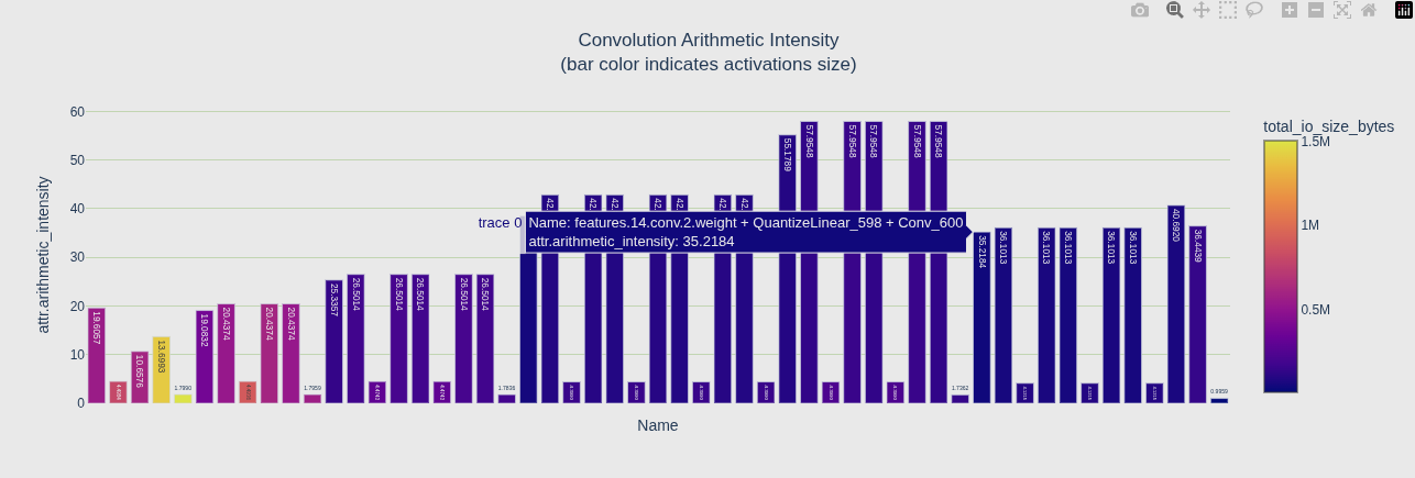
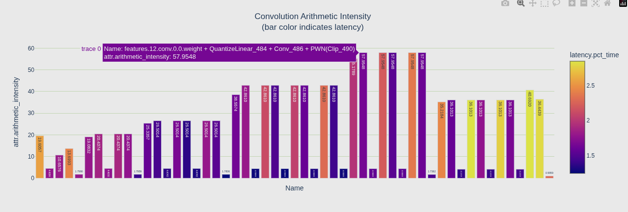
算术强度（Arithmetic Intensity）

定义：计算量 / 内存访问量（FLOPs / bytes）
含义：每访问一个字节能做多少计算
判断：
- 值越高 → 计算密度越大 → 容易被 GPU 算力瓶颈
- 值越低 → 瓶颈在内存带宽

图	颜色映射	回答的问题
第一个	`color='total_io_size_bytes'`	激活值大的卷积颜色深
第二个	`color='latency.pct_time'`	延迟高的卷积颜色深

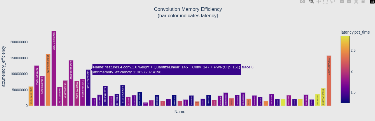
内存效率（Memory Efficiency）

定义：实际内存访问量 / 每毫秒可达到的内存带宽
公式：memory_efficiency = 实际内存访问(bytes) / (内存带宽(bytes/ms) × 执行时间(ms))
越高越好：说明充分利用了内存带宽

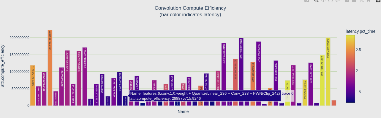
计算效率（Compute Efficiency）

定义：实际计算量 / 每毫秒可达到的峰值算力
公式：compute_efficiency = 实际FLOPs / (峰值算力(FLOPs/ms) × 执行时间(ms))
越高越好：说明充分利用了 GPU 算力

瓶颈判断

组合	结论
Memory 低、Compute 高	内存带宽瓶颈 --- 瓶颈在显存读写
Memory 高、Compute 低	计算瓶颈 --- 瓶颈在 GPU 算力
两者都高	正常，两边都被吃满了

图怎么看

颜色深（latency 高）= 该层延迟大，可能是瓶颈层
高延迟层 + Memory Efficiency 低 → 优化方向：减少内存访问或提高带宽
高延迟层 + Compute Efficiency 低 → 优化方向：提高计算密度或降低计算量

参考

deepseek

Tensorrt git 仓库