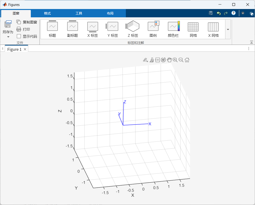
MATLAB机器人工具箱(RTB)超详细入门教程|五大核心实验脚本完整解析
目录
[1. 脚本核心用途](#1. 脚本核心用途)
[2. 核心代码逐段解析](#2. 核心代码逐段解析)
[3. 本实验运行](#3. 本实验运行)
[1. 脚本核心用途](#1. 脚本核心用途)
[2. 核心代码解析](#2. 核心代码解析)
[3. 本实验运行](#3. 本实验运行)
三、实验三:机器人姿态表示|旋转矩阵/欧拉角/RPY/四元数
[1. 脚本核心用途](#1. 脚本核心用途)
[2. 核心代码解析](#2. 核心代码解析)
[3. 本实验核心知识点](#3. 本实验核心知识点)
[4. 本实验运行](#4. 本实验运行)
[1. 脚本核心用途](#1. 脚本核心用途)
[2. 核心代码解析](#2. 核心代码解析)
[4. 本实验运行](#4. 本实验运行)
[五、实验五:机器人轨迹规划详解|tpoly、lspb、mtraj、ctraj 全解析](#五、实验五:机器人轨迹规划详解|tpoly、lspb、mtraj、ctraj 全解析)
[1. 脚本核心用途](#1. 脚本核心用途)
[2. 逐行代码详细解析](#2. 逐行代码详细解析)
[(1)一维五次多项式轨迹 tpoly](#(1)一维五次多项式轨迹 tpoly)
[(3)梯形速度轨迹 lspb](#(3)梯形速度轨迹 lspb)
[(4)多维向量轨迹插值 mtraj](#(4)多维向量轨迹插值 mtraj)
[(5)齐次位姿轨迹插值 ctraj](#(5)齐次位姿轨迹插值 ctraj)
[4. 四大轨迹算法对比总结](#4. 四大轨迹算法对比总结)
[5. 本实验运行](#5. 本实验运行)
📌 博客简介
本文基于 Peter Corke 官方 Robotics Toolbox for MATLAB(RTB) 五大入门示例脚本,从零拆解机器人建模、DH参数、轨迹规划、姿态表示、齐次坐标变换核心知识点。所有代码逐行解析、标注用途、用法与核心原理,适合机器人专业初学者、课程实验、毕设入门,可直接作为课程实验报告与学习笔记使用。
文件查找:
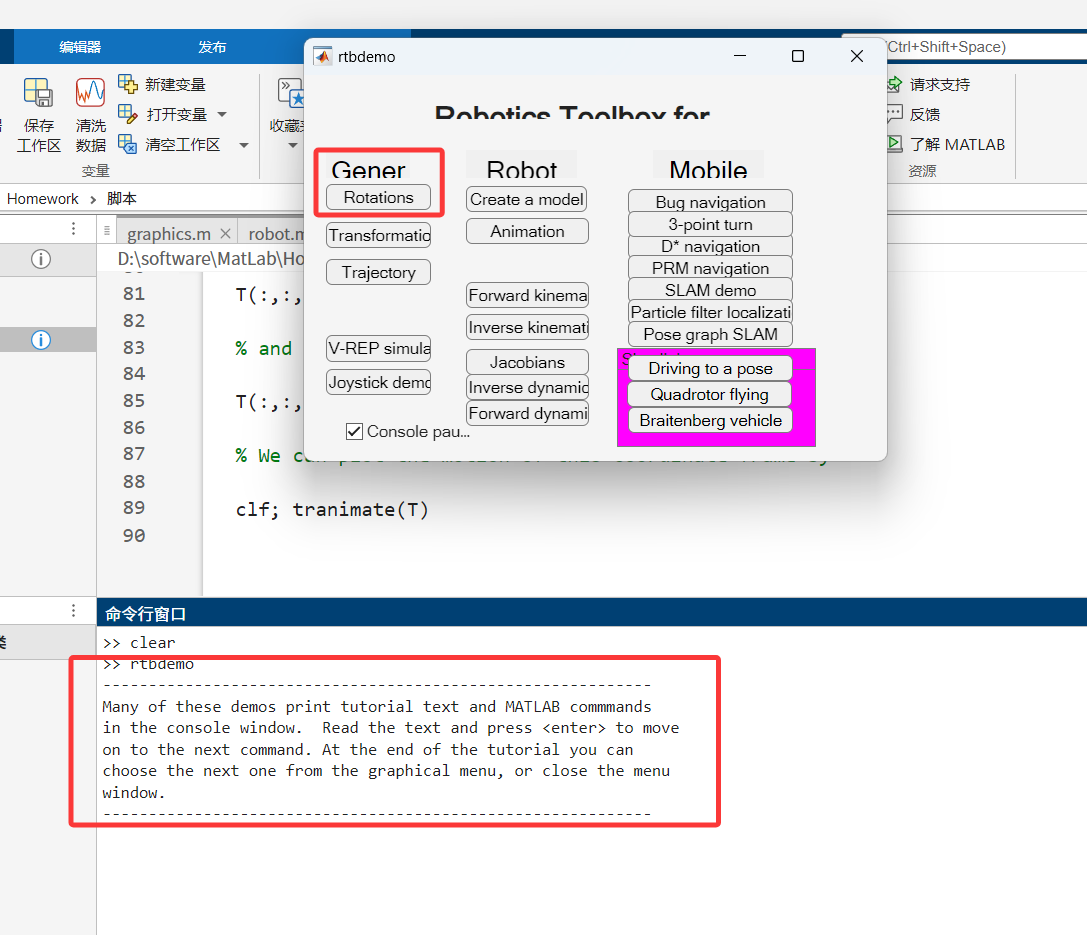
输入指令rtbdemo在终端,一直点击回车键(enter)就可进入此界面,点击Rotations可以在终端发现脚本路径,找到脚本路径文件,打开分析
bash
--- runscript <-- C:\Users\chujiacheng\AppData\Roaming\MathWorks\MATLAB Add-Ons\Toolboxes\Robotics Toolbox for MATLAB(2)\demos\rotation.m

In the field of robotics there are many possible ways of representing
orientations of which the most common are:
- orthonormal rotation matrices (3x3),
- three angles (1x3), and
- quaternions.

A rotation of pi/2 about the x-axis can be represented as an orthonormal rotation
matrix

>> R = rotx(pi/2)


R =

1.0000 0 0
0 0.9996 -0.0274
0 0.0274 0.9996


which we can see is a 3x3 matrix.

Such a matrix has the property that it's columns (and rows) are sets of orthogonal
unit vectors. The determinant of such a matrix is always 1

>> det(R)


ans =

1.0000


Let's create a more complex rotation
>> R = rotx(30, 'deg') * roty(50, 'deg') * rotz(10, 'deg')

------ done --------
**注:一定要顶置路径,**否则打不开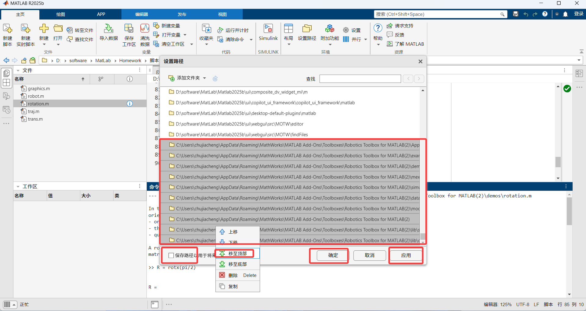
一、实验一:Puma560机械臂轨迹仿真与交互示教
1. 脚本核心用途
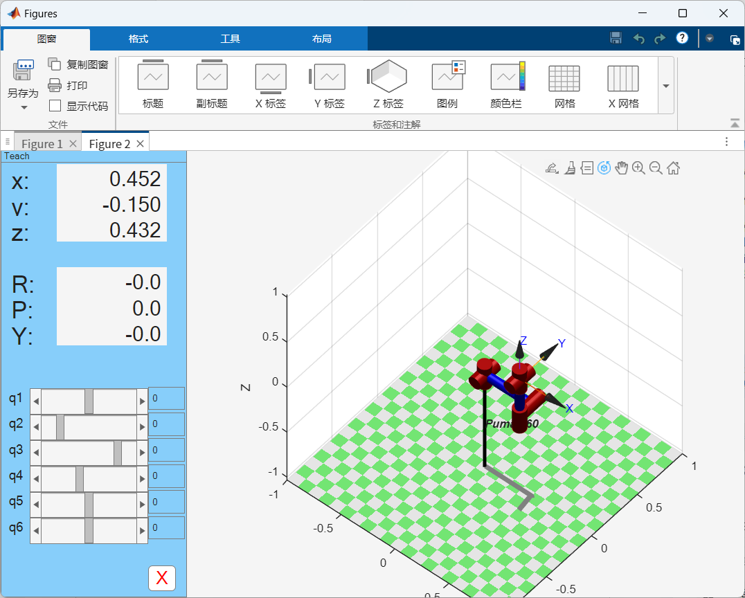
RTB 最经典入门案例,实现六自由度Puma560工业机械臂建模、轨迹规划、3D动画仿真、多机器人同场仿真、多视角观测、手动示教操控,是机器人轨迹与可视化入门必学代码。
2. 核心代码逐段解析
(1)加载官方Puma560机器人模型
Matlabmdl_puma560自动生成全局机械臂对象
p560,预定义两个关键位姿:
qz:零位姿态(机械臂竖直归位)
qr:标准收纳参考姿态
(2)生成时间序列与关节轨迹
Matlabt = [0:.05:2]'; % 0~2s,步长0.05s时间序列 q = jtraj(qz, qr, t); % 五次多项式关节平滑轨迹
jtraj为 RTB 核心轨迹函数,保证运动位置、速度、加速度连续,贴合工业机器人运动特性。(3)单机器人3D动画仿真
Matlabp560.plot(q);自动渲染机械臂骨架、末端坐标系、地面阴影,支持鼠标自由旋转观测视角。
(4)多机器人同窗口仿真
Matlabp560_2 = SerialLink(p560, 'name', 'another Puma', 'base', transl(-0.5, 0.5, 0) ) hold on p560_2.plot(q);克隆机械臂模型,修改基坐标位置,实现多机械臂同场景协同仿真。
(5)多窗口多视角同步观测
Matlabclf p560.plot(qr); figure p560.plot(qr); view(40,50) p560.plot(q)支持多窗口、不同视角同步动画,方便观察机械臂空间运动状态。
(6)手动示教与位姿读取
Matlabp560.teach() % 手动滑块控制各关节 p560.getpos() % 读取当前关节角度模拟工业示教盒,手动调试机械臂姿态,精准获取目标关节角度。
3. 本实验运行
Matlab
mdl_puma560
% The trajectory demonstration has shown how a joint coordinate trajectory
% may be generated
t = [0:.05:2]'; % generate a time vector
q = jtraj(qz, qr, t); % generate joint coordinate trajectory
% the overloaded function plot() animates a stick figure robot moving
% along a trajectory.
p560.plot(q);
% The drawn line segments do not necessarily correspond to robot links, but
% join the origins of sequential link coordinate frames.
%
% A small right-angle coordinate frame is drawn on the end of the robot to show
% the wrist orientation.
%
% A shadow appears on the ground which helps to give some better idea of the
% 3D object.
%
% This is a 3D plot so using the tools on the figure toolbar you can rotate the
% figure and change your viewpoint.
%--
% We can also place additional robots into a figure.
%
% Let's make a clone of the Puma robot, but change its name and base location
p560_2 = SerialLink(p560, 'name', 'another Puma', 'base', transl(-0.5, 0.5, 0) )
hold on
p560_2.plot(q);
% We can also have multiple views of the same robot
clf
p560.plot(qr);
figure
p560.plot(qr);
view(40,50)
% so now when we animate the robot, it moves in both views
p560.plot(q)
% Sometimes it's useful to be able to manually drive the robot around to
% get an understanding of how it works.
p560.teach()
% Use the sliders to control the robot (in fact both views). Hit the
% red X button when you are done.
% you can find the final joint angles of the robot you drove it to
p560.getpos()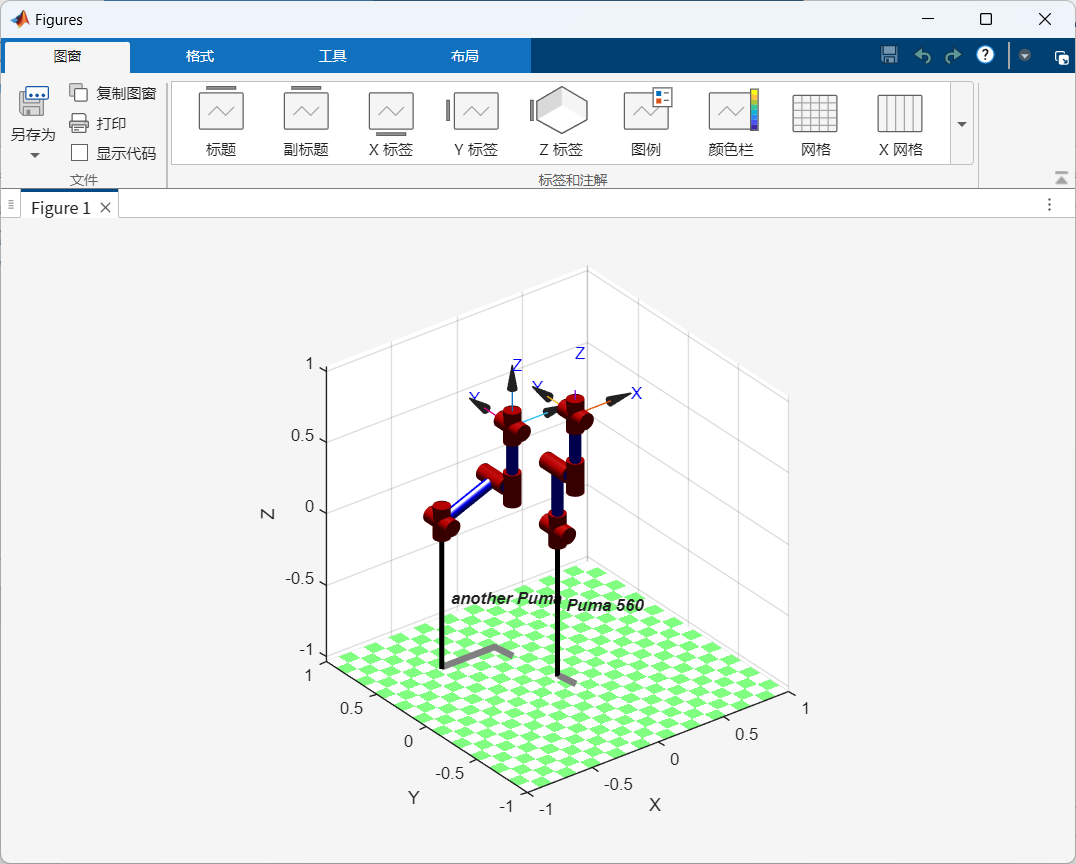
二、实验二:DH参数建模|二连杆机械臂从零建模+正运动学
1. 脚本核心用途
脱离官方模型,手动通过DH参数从零搭建二连杆串联机械臂,掌握连杆定义、机器人组装、单连杆变换、正运动学求解与模型可视化,是机器人运动学建模核心实验。
2. 核心代码解析
(1)自定义DH连杆
MatlabL1 = Link('d', 0, 'a', 1, 'alpha', pi/2) L2 = Link('d', 0, 'a', 1, 'alpha', 0)通过DH四参数(偏距d、杆长a、扭角alpha、转角theta)定义连杆结构。
(2)查看连杆属性与单连杆变换
Matlab
L1.a
L1.d
L1.isrevolute % 判断是否为转动关节
L1.A(0.2)    % 单连杆齐次变换矩阵
(3)组装串联机械臂
Matlab
bot = SerialLink([L1 L2], 'name', 'my robot')
bot.n % 获取机器人关节数量
(4)正运动学求解+可视化
Matlab
bot.fkine([0.1 0.2]) % 输入关节角,求解末端位姿矩阵
bot.plot([0.1 0.2])   % 3D绘制机械臂位形
3. 本实验运行
Matlab
L1 = Link('d', 0, 'a', 1, 'alpha', pi/2)

% The Link object we created has a number of properties
L1.a
L1.d

% and we determine that it is a revolute joint
L1.isrevolute

% For a given joint angle, say q=0.2 rad, we can determine the link transform
% matrix
L1.A(0.2)

% The second link is
L2 = Link('d', 0, 'a', 1, 'alpha', 0)

% Now we need to join these into a serial-link robot manipulator

bot = SerialLink([L1 L2], 'name', 'my robot')
% The displayed robot object shows a lot of details.  It also has a number of
% properties such as the number of joints
bot.n

% Given the joint angles q1 = 0.1 and q2 = 0.2 we can determine the pose of the
% robot's end-effector

bot.fkine([0.1 0.2])
% which is referred to as the forward kinematics of the robot.  This, and the
% inverse kinematics are covered in separate demos.

% Finally we can draw a stick figure of our robot

bot.plot([0.1 0.2])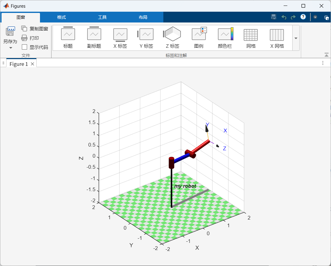
三、实验三:机器人姿态表示|旋转矩阵/欧拉角/RPY/四元数
1. 脚本核心用途
系统学习机器人四种主流姿态描述方式:旋转矩阵、轴角、欧拉角、RPY角、四元数,掌握相互转换、姿态叠加、求逆运算,解决姿态解算、万向锁认知问题。
2. 核心代码解析
(1)基础旋转矩阵生成与校验
Matlab
R = rotx(pi/2)  % 绕X轴旋转90°
det(R)          % 旋转矩阵行列式恒为1(正交矩阵特性)
(2)多轴复合旋转
Matlab
R = rotx(30, 'deg') * roty(50, 'deg') * rotz(10, 'deg')(3)姿态格式互转
Matlab
[theta,vec] = tr2angvec(R) % 旋转矩阵→轴角
eul = tr2eul(R)            % 旋转矩阵→Z-Y-Z欧拉角
rpy = tr2rpy(R)            % 旋转矩阵→X-Y-Z RPY横滚俯仰偏航角
(4)交互式姿态可视化
Matlab
tripleangle('rpy', 'wait')(5)四元数转换与运算
Matlab
q = Quaternion(R)  % 矩阵转四元数
q.R                % 四元数转回矩阵

q1 = Quaternion( rotx(pi/2) )
q2 = Quaternion( roty(pi/2) )
q1 * q2            % 姿态叠加
q1 * inv(q1)       % 姿态抵消(零旋转)
3. 本实验核心知识点
-
欧拉角:机械臂常用,存在万向锁缺陷
-
RPY角:移动机器人、无人机常用
-
四元数:无万向锁,适合姿态插值、实时解算
4. 本实验运行
Matlab
R = rotx(pi/2)
% which we can see is a 3x3 matrix.

% Such a matrix has the property that it's columns (and rows) are sets of orthogonal
% unit vectors.  The determinant of such a matrix is always 1

det(R)

% Let's create a more complex rotation

R = rotx(30, 'deg') * roty(50, 'deg') * rotz(10, 'deg')
% where this time we have specified the rotation angle in degrees.

% Any rotation can be expressed in terms of a single rotation about some axis
% in space

[theta,vec] = tr2angvec(R)
% where theta is the angle (in radians) and vec is unit vector representing the
% direction of the rotation axis.

% Commonly rotations are represented by Euler angles

eul = tr2eul(R)
% which are three angles such that R = rotz(a)*roty(b)*rotz(c), ie. the rotations
% required about the Z, then then the Y, then the Z axis.

% Rotations are also commonly represented by roll-pitch-yaw  angles

rpy = tr2rpy(R)
% which are three angles such that R = rotx(r)*roty(p)*rotz(y), ie. the rotations
% required about the X, then then the Y, then the Z axis.

% We can investigate the effects of rotations about different axes
% using this GUI based demonstration.  The menu buttons allow the rotation
% axes to be varied
%  *** close the window when you are done.
tripleangle('rpy', 'wait')

% The final useful form is the quaternion which comprises 4 numbers.  We can create
% a quaternion from an orthonormal matrix

q = Quaternion(R)
% where we can see that it comprises a scalar part and a vector part.  To convert back

q.R
% which is the same of the value of R we determined above.

% Quaternions are a class and the orientations they represent can be compounded, just
% as we do with rotation matrices by multiplication.

% First we create two quaternions

q1 = Quaternion( rotx(pi/2) )
q2 = Quaternion( roty(pi/2) )

% then the rotation of q1 followed by q2 is simply

q1 * q2

% We can also take the inverse of a Quaternion

q1 * inv(q1)
% which results in a null rotation (zero vector part)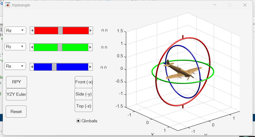
四、实验四:齐次坐标变换|平移、旋转、复合变换原理
1. 脚本核心用途
掌握机器人齐次变换矩阵 核心用法,实现平移、旋转、复合位姿变换,求解坐标系原点位置与姿态,验证空间变换乘法非交换性核心原理。
2. 核心代码解析
(1)基础平移、旋转变换
Matlab
transl(0.5, 0.0, 0.0)  % X轴平移0.5m齐次矩阵
troty(pi/2)            % 绕Y轴旋转90°
trotz(-pi/2)           % 绕Z轴顺时针旋转90°
(2)复合位姿变换
Matlab
t = transl(0.5, 0.0, 0.0) * troty(pi/2) * trotz(-pi/2)(3)求解新坐标系原点与姿态
Matlab
t * [0 0 0 1]'  % 计算新坐标系原点坐标
tr2eul(t)       % 提取欧拉角姿态
tr2rpy(t)       % 提取RPY姿态
(4)验证变换非交换性(重点)
Matlab
trotx(pi/2) * trotz(-pi/8)
trotz(-pi/8) * trotx(pi/2)
4. 本实验运行
Matlab
transl(0.5, 0.0, 0.0)

% a rotation of 90degrees about the Y axis by

troty(pi/2)

% and a rotation of -90degrees about the Z axis by

trotz(-pi/2)

%  these may be concatenated by multiplication

t = transl(0.5, 0.0, 0.0) * troty(pi/2) * trotz(-pi/2)

%
% If this transformation represented the origin of a new coordinate frame with respect
% to the world frame origin (0, 0, 0), that new origin would be given by

t * [0 0 0 1]'

% the orientation of the new coordinate frame may be expressed in terms of
% Euler angles

tr2eul(t)

% or roll/pitch/yaw angles

tr2rpy(t)

% It is important to note that tranform multiplication is in general not
% commutative as shown by the following example

trotx(pi/2) * trotz(-pi/8)
trotz(-pi/8) * trotx(pi/2)
运行结果
bash
ans =

    1.0000         0         0    0.5000
         0    1.0000         0         0
         0         0    1.0000         0
         0         0         0    1.0000


ans =

    0.9996         0    0.0274         0
         0    1.0000         0         0
   -0.0274         0    0.9996         0
         0         0         0    1.0000


ans =

    0.9996    0.0274         0         0
   -0.0274    0.9996         0         0
         0         0    1.0000         0
         0         0         0    1.0000


t =

    0.9992    0.0274    0.0274    0.5000
   -0.0274    0.9996         0         0
   -0.0274   -0.0008    0.9996         0
         0         0         0    1.0000


ans =

    0.5000
         0
         0
    1.0000


ans =

         0    0.0274   -0.0274


ans =

   -0.0008    0.0274   -0.0274


ans =

    1.0000    0.0069         0         0
   -0.0069    0.9996   -0.0274         0
   -0.0002    0.0274    0.9996         0
         0         0         0    1.0000


ans =

    1.0000    0.0069   -0.0002         0
   -0.0069    0.9996   -0.0274         0
         0    0.0274    0.9996         0
         0         0         0    1.0000
五、实验五:机器人轨迹规划详解|tpoly、lspb、mtraj、ctraj 全解析
1. 脚本核心用途
本脚本为 RTB 官方轨迹规划核心案例,系统讲解机器人一维多项式轨迹、梯形速度轨迹、多维向量轨迹、齐次位姿轨迹四种主流插值算法。可输出位置、速度、加速度曲线,实现从一维标量→多维坐标→完整位姿的平滑轨迹生成,是机械臂轨迹规划、运动仿真的核心基础。
2. 逐行代码详细解析
(1)一维五次多项式轨迹 tpoly
Matlabp0 = -1; p1 = 2; p = tpoly(p0, p1, 50); about p plot(p)功能用途 :生成五次多项式一维平滑轨迹。强制起点、终点速度、加速度均为0,运动启停无冲击,是机器人最基础的平滑轨迹算法。
参数含义 :
tpoly(起点, 终点, 总步数),输出每一步的位置序列。(2)输出轨迹完整运动参数(位置/速度/加速度)
Matlab[p,pd,pdd] = tpoly(p0, p1, 50); subplot(3,1,1); plot(p); xlabel('Time'); ylabel('p'); subplot(3,1,2); plot(pd); xlabel('Time'); ylabel('pd'); subplot(3,1,3); plot(pdd); xlabel('Time'); ylabel('pdd');可同时返回:
p位置、pd速度、pdd加速度,三图联动展示完整运动特性,适合轨迹性能分析。(3)梯形速度轨迹 lspb
Matlab[p,pd,pdd] = lspb(p0, p1, 50); subplot(3,1,1); plot(p); xlabel('Time'); ylabel('p'); subplot(3,1,2); plot(pd); xlabel('Time'); ylabel('pd'); subplot(3,1,3); plot(pdd); xlabel('Time'); ylabel('pdd');核心优势 :
lspb为梯形速度曲线,加速→匀速→减速三段式运动,速度利用率更高、运动效率优于纯五次多项式,更贴合工业机器人高速搬运场景。(4)多维向量轨迹插值 mtraj
Matlabp = mtraj(@tpoly, [0 1 2], [2 1 0], 50); about p clf; plot(p)功能用途 :将一维轨迹算法扩展到多维向量,可用于3D坐标、欧拉角、多关节角度同步插值。
参数说明 :绑定 tpoly 算法,起点向量
[0 1 2]、终点向量[2 1 0],50步平滑插值,各维度独立平滑运动。(5)齐次位姿轨迹插值 ctraj
Matlabp = mtraj(@tpoly, [0 1 2], [2 1 0], 50); about p clf; plot(p)核心功能 :机器人完整位姿插值(位置+姿态同时平滑变化)。
输入两个4×4齐次变换矩阵,
ctraj实现位置平移、姿态旋转的同步平滑过渡,生成4×4×步数的三维轨迹矩阵。
tranimate(T):直接动画演示坐标系从起始位姿到终止位姿的连续运动过程,可视化效果直观。
4. 四大轨迹算法对比总结
-
tpoly:五次多项式,启停平稳、无冲击,适合低速精密运动,速度利用率低。
-
lspb:梯形速度曲线,含匀速段,运动效率高,工业机器人常用。
-
mtraj:多维轨迹插值,适配多关节、三维坐标同步运动。
-
ctraj:位姿级轨迹插值,实现位置+姿态整体平滑过渡,用于末端轨迹仿真。
5. 本实验运行
Matlab
p0 = -1;
p1 = 2;
% and a smooth path from p0 to p1 in 50 time steps is given by
p = tpoly(p0, p1, 50);
about p
% which we see has 50 rows. We can plot this
plot(p)
% and see that it does indeed move smoothly from p0 to p1 and that the initial
% and final derivative (and second derivative) is zero.
% We can also get the velocity and acceleration
[p,pd,pdd] = tpoly(p0, p1, 50);
subplot(3,1,1); plot(p); xlabel('Time'); ylabel('p');
subplot(3,1,2); plot(pd); xlabel('Time'); ylabel('pd');
subplot(3,1,3); plot(pdd); xlabel('Time'); ylabel('pdd');
% This path is a 5th order polynomial and it suffers from the disadvantage that
% the velocity is mostly below the maximum possible value. An alternative is
[p,pd,pdd] = lspb(p0, p1, 50);
subplot(3,1,1); plot(p); xlabel('Time'); ylabel('p');
subplot(3,1,2); plot(pd); xlabel('Time'); ylabel('pd');
subplot(3,1,3); plot(pdd); xlabel('Time'); ylabel('pdd');
% which we see has a trapezoidal velocity profile.
% Frequently the start and end values are vectors, not scalars, perhaps a 3D
% position or Euler angles. In this case we apply the scalar trajectory function
% to a vector with
p = mtraj(@tpoly, [0 1 2], [2 1 0], 50);
about p
% and p again has one row per time step, and one column per vector dimension
clf; plot(p)
%---
% Finally, we may wish to interpolate poses. We will define a start and end pose
T0 = transl(0.4, 0.2, 0) * trotx(pi);
T1 = transl(-0.4, -0.2, 0.3) * troty(pi/2) * trotz(-pi/2);
% and a smooth sequence between them in 50 steps is
T = ctraj(T0, T1, 50);
about T
% which is a 4x4x50 matrix. The first pose is
T(:,:,1)
% and the 10th pose is
T(:,:,10)
% We can plot the motion of this coordinate frame by
clf; tranimate(T)