用rpart算法预测汽车是自动挡还是手动挡(am 变量),这是一个二分类任务。
R
# ==================== 1. 安装并加载需要的包 ====================
# rpart:构建决策树模型
# rpart.plot:画出漂亮的决策树
# caret:用于模型评估
#install.packages(c("rpart", "rpart.plot", "caret"))  # 第一次运行需要安装

library(rpart)       # 决策树算法包
library(rpart.plot)  # 决策树可视化包
library(caret)       # 模型评估工具

# ==================== 2. 加载并查看 mtcars 数据集 ====================
data(mtcars)  # 加载R自带数据集

# 查看数据集前几行
head(mtcars)

# 查看数据集结构
# 变量说明:
# am = 0 自动挡,1 手动挡(我们要预测的目标)
# mpg = 油耗,disp = 排量,hp = 马力,wt = 车重 ...
str(mtcars)

# 把分类标签 am 转换成因子型(决策树分类任务必须是因子)
mtcars$am <- as.factor(mtcars$am)
levels(mtcars$am) <- c("自动挡", "手动挡")  # 给类别起名字,方便看结果
训练模型
R
# ==================== 3. 划分训练集(70%) 和 测试集(30%) ====================
set.seed(123)  # 固定随机种子,结果可复现

# 随机抽取70%的数据作为训练集
train_index <- sample(1:nrow(mtcars), 0.7*nrow(mtcars))
train_data <- mtcars[train_index, ]   # 训练集
test_data  <- mtcars[-train_index, ]  # 测试集

# ==================== 4. 训练决策树模型 ====================
# 公式:am ~ .  表示用所有其他变量预测 am(自动挡/手动挡)
# method = "class" 表示做分类任务
tree_model <- rpart(
  formula = am ~ .,   # 目标变量 ~ 所有特征
  data = train_data,  # 训练数据
  method = "class"    # 分类模型
)

# 查看决策树规则(非常重要!能看到模型是怎么判断的)
print(tree_model)
n= 22
node), split, n, loss, yval, (yprob)
* denotes terminal node
-
root 22 11 0 (0.5000000 0.5000000)
-
wt>=2.965 13 2 0 (0.8461538 0.1538462) *
-
wt< 2.965 9 0 1 (0.0000000 1.0000000) *
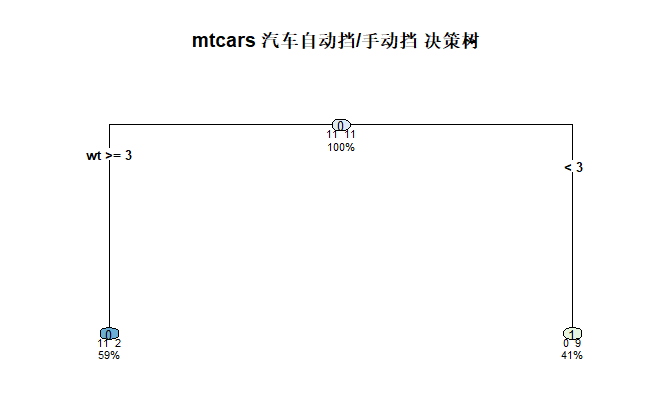
- 车重(wt)< 2.965 → 大概率是手动挡
- 车重(wt)≥ 2.965 → 大概率是自动挡
R
# 查看详细模型信息
summary(tree_model)
Call:
rpart(formula = am ~ ., data = train_data, method = "class")
n= 22
CP nsplit rel error xerror xstd
1 0.8181818 0 1.0000000 1.3636364 0.1986052
2 0.0100000 1 0.1818182 0.6363636 0.1986052
Variable importance
wt disp mpg cyl hp drat
22 20 17 15 15 12
Node number 1: 22 observations, complexity param=0.8181818
predicted class=0 expected loss=0.5 P(node) =1
class counts: 11 11
probabilities: 0.500 0.500
left son=2 (13 obs) right son=3 (9 obs)
Primary splits:
wt < 2.965 to the right, improve=7.615385, (0 missing)
disp < 130.9 to the right, improve=6.285714, (0 missing)
drat < 3.385 to the left, improve=5.133333, (0 missing)
gear < 3.5 to the left, improve=5.133333, (0 missing)
mpg < 19.45 to the left, improve=4.454545, (0 missing)
Surrogate splits:
disp < 130.9 to the right, agree=0.955, adj=0.889, (0 split)
mpg < 19.45 to the left, agree=0.909, adj=0.778, (0 split)
cyl < 5 to the right, agree=0.864, adj=0.667, (0 split)
hp < 118 to the right, agree=0.864, adj=0.667, (0 split)
drat < 4 to the left, agree=0.818, adj=0.556, (0 split)
Node number 2: 13 observations
predicted class=0 expected loss=0.1538462 P(node) =0.5909091
class counts: 11 2
probabilities: 0.846 0.154
Node number 3: 9 observations
predicted class=1 expected loss=0 P(node) =0.4090909
class counts: 0 9
probabilities: 0.000 1.000
可视化
R
# ==================== 5. 决策树可视化(最直观!) ====================
# 画出决策树
rpart.plot(
  tree_model,
  main = "mtcars 汽车自动挡/手动挡 决策树",
  type = 4,            # 树的样式
  extra = 101,         # 显示分类比例
  under = TRUE,        # 标签放下方
  cex = 0.8            # 字体大小
)
R
# ==================== 6. 模型预测 ====================
# 对测试集进行预测
pred <- predict(tree_model, test_data, type = "class")

# 查看预测结果 vs 真实结果
cat("预测结果:\n")
print(pred)
cat("\n真实结果:\n")
print(test_data$am)
预测结果:
> print(pred)
Mazda RX4 Mazda RX4 Wag Hornet 4 Drive Valiant
1 1 0 0
Merc 450SE Merc 450SL Lincoln Continental Toyota Corona
0 0 0 1
Camaro Z28 Pontiac Firebird
0 0
Levels: 0 1
> cat("\n真实结果:\n")
真实结果:
> print(test_data$am)
1 1 1 0 0 0 0 0 0 0 0
混淆矩阵
R
# ==================== 7. 模型评估:计算准确率 ====================
# 混淆矩阵
test_data$am = as.factor(test_data$am)
cm <- confusionMatrix(pred, test_data$am)
print(cm)
Confusion Matrix and Statistics
Reference
Prediction 0 1
0 7 0
1 1 2
Accuracy : 0.9
95% CI : (0.555, 0.9975)
No Information Rate : 0.8
P-Value Acc \> NIR : 0.3758
Kappa : 0.7368
Mcnemar's Test P-Value : 1.0000
Sensitivity : 0.8750
Specificity : 1.0000
Pos Pred Value : 1.0000
Neg Pred Value : 0.6667
Prevalence : 0.8000
Detection Rate : 0.7000
Detection Prevalence : 0.7000
Balanced Accuracy : 0.9375
'Positive' Class : 0