1. 前言
本文记录一次 YOLO26 模型的完整测试流程,主要包括环境验证、官方模型下载、测试模型预测、自定义数据集训练、模型导出为 ONNX、.pt 与 .onnx 推理结果对比,以及使用 ONNX Runtime 手动验证导出的 ONNX 模型。
这篇文章的目标不是系统分析 YOLO26 的网络结构,而是从工程实践角度梳理一套可复现的测试流程。整个流程可以概括为:
模型环境验证 → 官方模型预测 → 自定义数据训练 → 模型导出 ONNX → PT 与 ONNX 结果对比 → ONNX Runtime 独立推理验证。
这样做的意义在于,不能只看模型能训练、能导出,还需要确认导出的模型在不同推理后端下结果一致。尤其在后续进入 RKNN、TensorRT、OpenVINO 或其他端侧部署前,ONNX Runtime 是一个非常重要的中间验证环节。
2. YOLO26 简要说明
YOLO26 是 Ultralytics YOLO 系列中的新一代目标检测模型,仍然延续了 Ultralytics 统一接口的使用方式,可以通过 YOLO() 完成模型加载、训练、验证、预测和导出。Ultralytics 官方文档说明,YOLO26 面向部署效率进行了优化,包括原生端到端 NMS-free 推理、移除 DFL 回归结构、轻量化检测头以及更适合导出的融合模型结构。
从工程使用角度看,YOLO26 的一个明显变化是导出的 ONNX 输出形式与传统 YOLO 模型不同。传统 YOLO 模型常见输出可能是类似 [1, 84, 8400] 的原始检测头结果,需要额外进行 decode、置信度筛选和 NMS。而本文测试的 YOLO26 ONNX 模型输出为:
[1, 300, 6]这个输出更接近最终检测结果格式,可以理解为最多输出 300 个检测目标,每个目标包含 6 个参数。
用数学形式表示,模型输出为:
其中:
1   表示 batch size,即一次输入 1 张图片;
300 表示最多输出 300 个检测结果;
6   表示每个检测结果包含 6 个参数。
每个检测结果的 6 个参数可以表示为:
含义如下:
x1       检测框左上角 x 坐标;
y1       检测框左上角 y 坐标;
x2       检测框右下角 x 坐标;
y2       检测框右下角 y 坐标;
score    检测置信度;
class_id 类别编号。
因此,对于该模型而言,传统 YOLO 中最复杂的 decode 和 NMS 后处理已经大幅简化。但这并不意味着完全不需要预处理和后处理。输入端仍然需要完成 resize、letterbox、颜色通道转换、归一化和维度转换;输出端仍然需要完成置信度过滤、类别映射、坐标还原和结果绘制。
3. 测试环境
本文测试环境如下:
操作系统:Windows
Python:3.8.19
Ultralytics:8.4.60
PyTorch:2.1.0+cu118
ONNX:1.14.1
ONNX Runtime:1.18.1
GPU:NVIDIA GeForce RTX 3060 Ti 8GB
CUDA:可用
训练日志中可以看到 GPU 被正常识别:
Ultralytics 8.4.60 Python-3.8.19 torch-2.1.0+cu118 CUDA:0 (NVIDIA GeForce RTX 3060 Ti, 8192MiB)ONNX Runtime 独立推理时,本文使用的是 CPU 后端:
Using ONNX Runtime 1.18.1 with CPUExecutionProvider这里需要说明一点:训练时使用 GPU,ONNX Runtime 验证时使用 CPU,是为了验证模型在通用 ONNX 推理后端上的可用性。
4. YOLO26 下载与版本验证
Ultralytics 官方文档说明,可以直接使用 YOLO("yolo26n.pt") 加载官方模型,如果本地没有对应权重文件,程序会自动尝试下载。YOLO26 也支持通过 Ultralytics 的统一接口导出为 ONNX 等格式。
在实际测试中,建议先做两件事。
第一,确认当前导入的 ultralytics 包来自哪里。因为如果项目目录下本身存在一个 ultralytics 源码文件夹,那么 Python 会优先导入当前项目路径下的源码,而不是虚拟环境 site-packages 中安装的版本。
第二,确认 Ultralytics 版本。本文使用版本为:
Ultralytics 8.4.60这一步很重要,因为 YOLO26 属于较新的模型,较旧版本的 Ultralytics 可能无法正常识别模型结构或导出格式。
验证代码:
python
import ultralytics
from ultralytics import YOLO

print("ultralytics 导入路径:")
print(ultralytics.__file__)

try:
    print("ultralytics 版本:", ultralytics.__version__)
except Exception as e:
    print("无法读取版本:", e)

model = YOLO("yolo26n.pt")
# print(model)
测试结果:
ultralytics 导入路径:
D:\Pycharm_project\Yolo26\ultralytics\init.py
ultralytics 版本: 8.4.60
5. 官方模型预测测试
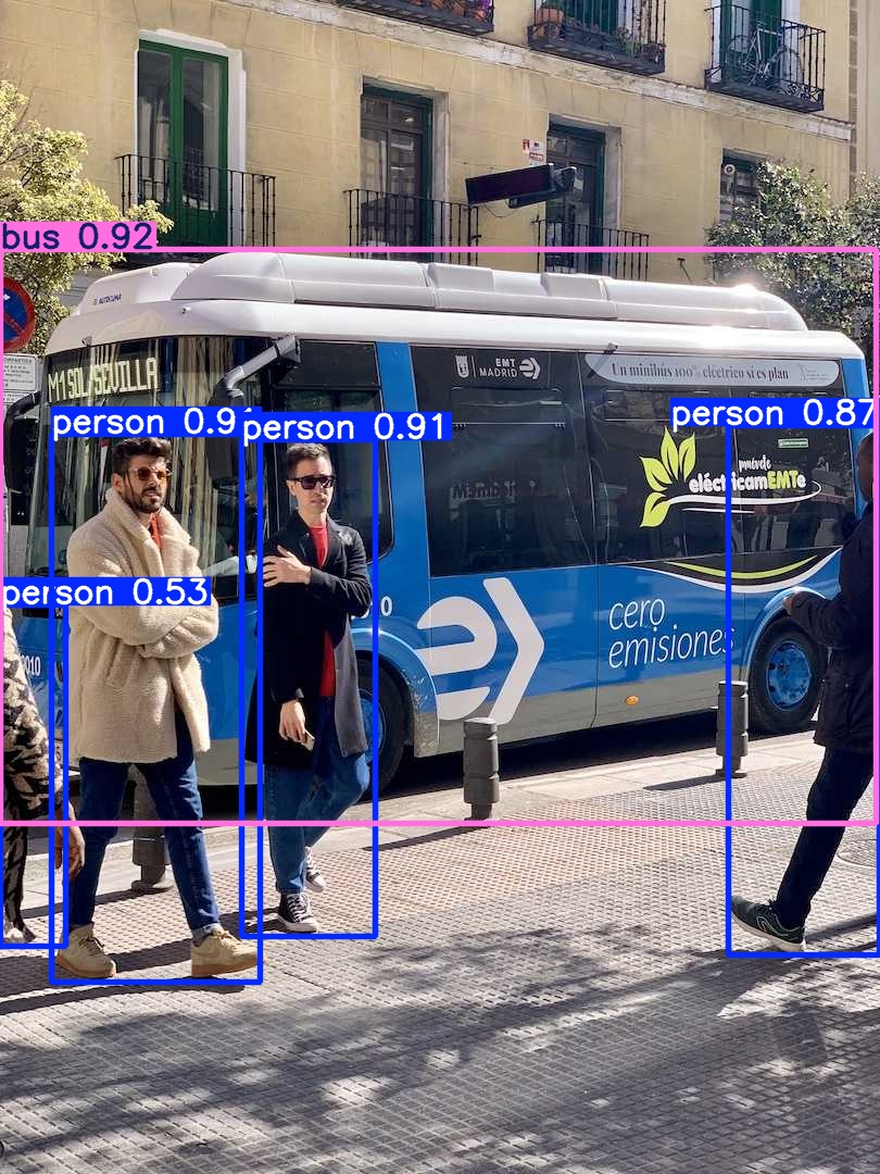
在完成环境验证后,首先使用官方 yolo26n.pt 模型对测试图片进行预测。测试图片来自 Ultralytics 项目中的 assets 目录。
python
from ultralytics import YOLO
import os

def main():
    model_path = "yolo26n.pt"
    image_path = r"D:\Pycharm_project\Yolo26\ultralytics\assets"

    model = YOLO(model_path)

    results = model.predict(
        source=image_path,
        imgsz=640,
        conf=0.25,
        device="cpu",
        save=True,
        show=False
    )

    # 打印本次结果保存目录
    if len(results) > 0:
        print("\n预测结果保存目录:")
        print(results[0].save_dir)

    # 按图片分别打印检测结果
    for i, result in enumerate(results):
        image_name = os.path.basename(result.path)

        print("\n" + "=" * 80)
        print(f"第 {i + 1} 张图片:{image_name}")
        print(f"原始图片路径:{result.path}")
        print("=" * 80)

        if result.boxes is None or len(result.boxes) == 0:
            print("未检测到目标")
            continue

        for j, box in enumerate(result.boxes):
            cls_id = int(box.cls[0])
            conf = float(box.conf[0])
            x1, y1, x2, y2 = box.xyxy[0].tolist()

            print(
                f"目标 {j + 1}: "
                f"类别={result.names[cls_id]}, "
                f"置信度={conf:.3f}, "
                f"框=[{x1:.1f}, {y1:.1f}, {x2:.1f}, {y2:.1f}]"
            )

    print("\n预测完成。")
    # input("按回车键退出...")


if __name__ == "__main__":
    main()
测试结果:
预测结果保存目录:
D:\Pycharm_project\Yolo26\runs\detect\predict
================================================================================
第 1 张图片:bus.jpg
原始图片路径:D:\Pycharm_project\Yolo26\ultralytics\assets\bus.jpg
================================================================================
目标 1: 类别=bus, 置信度=0.924, 框=0.0, 229.4, 806.1, 757.1
目标 2: 类别=person, 置信度=0.913, 框=222.5, 404.9, 345.4, 861.6
目标 3: 类别=person, 置信度=0.905, 框=47.7, 399.3, 239.3, 903.0
目标 4: 类别=person, 置信度=0.870, 框=670.7, 391.5, 809.8, 879.0
目标 5: 类别=person, 置信度=0.535, 框=0.1, 556.7, 60.0, 870.1
================================================================================
第 2 张图片:zidane.jpg
原始图片路径:D:\Pycharm_project\Yolo26\ultralytics\assets\zidane.jpg
================================================================================
目标 1: 类别=person, 置信度=0.915, 框=744.6, 40.5, 1150.3, 711.8
目标 2: 类别=person, 置信度=0.910, 框=120.4, 201.7, 981.5, 713.7
目标 3: 类别=tie, 置信度=0.527, 框=433.2, 430.7, 525.6, 714.9
预测完成。
6. 自定义数据集训练
完成官方模型测试后,使用自定义 AVS 数据集训练 YOLO26。数据集配置文件为:
D:\Pycharm_project\Yolo26\AVS_dataset\data.yamldata.yaml:
python
path:  D:\Pycharm_project\Yolo26\AVS_dataset
train: D:\Pycharm_project\Yolo26\AVS_dataset\images\train
val:  D:\Pycharm_project\Yolo26\AVS_dataset\images\val
test:    # test images (optional)

nc: 2
# Classes
names:
  0: AVS
  1: handle
该数据集包含两个类别:
AVS
handle
训练时使用官方 yolo26n.pt 作为预训练权重。训练参数如下:
epochs=200
imgsz=640
batch=16
device=0
project=D:\Pycharm_project\Yolo26\runs
name=AVS_Yolo26
训练启动后,日志中出现:
Overriding model.yaml nc=80 with nc=2这说明原始 COCO 80 类模型的检测头被替换为当前数据集的 2 类检测头。
7. 训练结果
训练完成后,模型自动验证 best.pt,最终验证日志如下:
Validating D:\Pycharm_project\Yolo26\runs\AVS_Yolo26\weights\best.pt...
YOLO26n summary (fused): 122 layers, 2,375,226 parameters, 0 gradients

Class     Images  Instances      Box(P          R      mAP50  mAP50-95)
all        135        135      0.987      0.993       0.99      0.916
AVS         67         67      0.977          1      0.995      0.885
handle      68         68      0.998      0.985      0.985      0.946

Speed: 0.4ms preprocess, 2.4ms inference, 0.0ms loss, 0.2ms postprocess per image
整体结果如下:
Precision = 0.987
Recall = 0.993
mAP50 = 0.990
mAP50-95 = 0.916
Precision 表示预测出来的目标中有多少是真实目标;Recall 表示真实目标中有多少被模型检测出来;mAP 则用于综合衡量检测精度。
mAP 可以简化表示为:
其中:
N    表示类别数量;
AP_i 表示第 i 个类别的 Average Precision。
从结果看,两个类别的检测效果都比较好。其中 AVS 类别的召回率达到 1.000,handle 类别的 mAP50-95 达到 0.946。
8. 导出 ONNX 模型
训练完成后,将 .pt 模型导出为 ONNX。Ultralytics 官方 Export 文档说明,YOLO26 支持通过 Python API 或 CLI 导出为 ONNX 格式,并且还支持 TensorRT、CoreML、OpenVINO、TFLite 等多种部署格式。
本文首先对官方 yolo26n.pt 进行了 ONNX 导出测试。导出日志如下:
ONNX: starting export with onnx 1.14.1 opset 17...
ONNX: slimming with onnxslim 0.1.94...
ONNX: export success  1.9s, saved as 'D:\Pycharm_project\Yolo26\yolo26n.onnx' (9.5 MB)
这里有几个关键信息。
第一,ONNX opset 使用的是 17。
第二,onnxslim 已经正常工作:
ONNX: slimming with onnxslim 0.1.94...之前没有安装 onnxslim 时,导出也可以成功,但会出现简化失败提示。安装后重新导出,ONNX 模型结构更干净。
为了确认 ONNX 导出是否正确,使用同一张测试图片分别调用 .pt 和 .onnx 模型进行预测。
测试代码:
python
from ultralytics import YOLO
import os

def print_results(model_name, results):
    print("\n" + "=" * 80)
    print(model_name)
    print("=" * 80)

    for result in results:
        image_name = os.path.basename(result.path)
        print(f"\n图片:{image_name}")

        if result.boxes is None or len(result.boxes) == 0:
            print("未检测到目标")
            continue

        for i, box in enumerate(result.boxes):
            cls_id = int(box.cls[0])
            conf = float(box.conf[0])
            x1, y1, x2, y2 = box.xyxy[0].tolist()

            print(
                f"目标 {i + 1}: "
                f"类别={result.names[cls_id]}, "
                f"置信度={conf:.3f}, "
                f"框=[{x1:.1f}, {y1:.1f}, {x2:.1f}, {y2:.1f}]"
            )


def main():
    image_path = r"D:\Pycharm_project\Yolo26\ultralytics\assets\bus.jpg"

    pt_model = YOLO(r"D:\Pycharm_project\Yolo26\yolo26n.pt")
    onnx_model = YOLO(r"D:\Pycharm_project\Yolo26\yolo26n.onnx")

    pt_results = pt_model.predict(
        source=image_path,
        imgsz=640,
        conf=0.25,
        device="cpu",
        save=True,
        project=r"D:\Pycharm_project\Yolo26\runs\compare",
        name="pt",
        exist_ok=True
    )

    onnx_results = onnx_model.predict(
        source=image_path,
        imgsz=640,
        conf=0.25,
        device="cpu",
        save=True,
        project=r"D:\Pycharm_project\Yolo26\runs\compare",
        name="onnx",
        exist_ok=True
    )

    print_results("PyTorch .pt 结果", pt_results)
    print_results("ONNX 结果", onnx_results)

    print("\n.pt 保存目录:", pt_results[0].save_dir)
    print(".onnx 保存目录:", onnx_results[0].save_dir)


if __name__ == "__main__":
    main()
测试图片为:
D:\Pycharm_project\Yolo26\ultralytics\assets\bus.jpg.pt 模型推理结果如下:
目标 1: 类别=bus,    置信度=0.924, 框=[0.0, 229.4, 806.1, 757.1]
目标 2: 类别=person, 置信度=0.913, 框=[222.5, 404.9, 345.4, 861.6]
目标 3: 类别=person, 置信度=0.905, 框=[47.7, 399.3, 239.3, 903.0]
目标 4: 类别=person, 置信度=0.870, 框=[670.7, 391.5, 809.8, 879.0]
目标 5: 类别=person, 置信度=0.535, 框=[0.1, 556.7, 60.0, 870.1]
.onnx 模型推理结果如下:
目标 1: 类别=bus,    置信度=0.925, 框=[5.6, 228.9, 807.2, 749.2]
目标 2: 类别=person, 置信度=0.915, 框=[46.6, 398.7, 237.0, 901.7]
目标 3: 类别=person, 置信度=0.899, 框=[223.1, 405.3, 345.2, 863.1]
目标 4: 类别=person, 置信度=0.860, 框=[668.6, 391.2, 810.0, 879.7]
目标 5: 类别=person, 置信度=0.525, 框=[0.0, 553.8, 64.8, 874.0]
从结果看,二者检测到的目标类别和数量一致,均为:
4 persons, 1 bus置信度非常接近。
可以认为.pt 与 .onnx 推理结果一致性较好。
9. 使用 ONNX Runtime 独立推理验证
完成 .pt 与 .onnx 对比后,进一步使用 ONNX Runtime 独立推理,不再依赖 Ultralytics 的 model.predict()。
测试代码:
python
import cv2
import numpy as np
import onnxruntime as ort
import os
import time


# COCO 80 类
# COCO_NAMES = [
#     "person", "bicycle", "car", "motorcycle", "airplane", "bus", "train", "truck",
#     "boat", "traffic light", "fire hydrant", "stop sign", "parking meter", "bench",
#     "bird", "cat", "dog", "horse", "sheep", "cow", "elephant", "bear", "zebra",
#     "giraffe", "backpack", "umbrella", "handbag", "tie", "suitcase", "frisbee",
#     "skis", "snowboard", "sports ball", "kite", "baseball bat", "baseball glove",
#     "skateboard", "surfboard", "tennis racket", "bottle", "wine glass", "cup",
#     "fork", "knife", "spoon", "bowl", "banana", "apple", "sandwich", "orange",
#     "broccoli", "carrot", "hot dog", "pizza", "donut", "cake", "chair", "couch",
#     "potted plant", "bed", "dining table", "toilet", "tv", "laptop", "mouse",
#     "remote", "keyboard", "cell phone", "microwave", "oven", "toaster", "sink",
#     "refrigerator", "book", "clock", "vase", "scissors", "teddy bear",
#     "hair drier", "toothbrush"
# ]

COCO_NAMES = [
     "AVS", "handle"
]


def letterbox(image, new_shape=(640, 640), color=(114, 114, 114)):
    """
    等比例缩放图片,并填充到指定大小。
    """
    h, w = image.shape[:2]
    new_h, new_w = new_shape

    r = min(new_w / w, new_h / h)

    resized_w = int(round(w * r))
    resized_h = int(round(h * r))

    dw = new_w - resized_w
    dh = new_h - resized_h

    dw /= 2
    dh /= 2

    resized = cv2.resize(
        image,
        (resized_w, resized_h),
        interpolation=cv2.INTER_LINEAR
    )

    top = int(round(dh - 0.1))
    bottom = int(round(dh + 0.1))
    left = int(round(dw - 0.1))
    right = int(round(dw + 0.1))

    padded = cv2.copyMakeBorder(
        resized,
        top,
        bottom,
        left,
        right,
        cv2.BORDER_CONSTANT,
        value=color
    )

    return padded, r, (left, top)


def preprocess(image_path, input_size=(640, 640)):
    """
    预处理:
    1. 读取图片
    2. letterbox 到 640x640
    3. BGR 转 RGB
    4. 归一化到 0~1
    5. HWC 转 CHW
    6. 增加 batch 维度
    """
    image = cv2.imread(image_path)

    if image is None:
        raise FileNotFoundError(f"无法读取图片: {image_path}")

    original_image = image.copy()

    img, ratio, pad = letterbox(
        image,
        new_shape=input_size
    )

    img = cv2.cvtColor(img, cv2.COLOR_BGR2RGB)
    img = img.astype(np.float32) / 255.0
    img = np.transpose(img, (2, 0, 1))
    img = np.expand_dims(img, axis=0)
    img = np.ascontiguousarray(img)

    return img, original_image, ratio, pad


def scale_boxes(box, ratio, pad, original_shape):
    """
    将 640x640 输入尺度下的检测框还原到原图尺度。
    box: [x1, y1, x2, y2]
    """
    left, top = pad

    x1, y1, x2, y2 = box

    x1 = (x1 - left) / ratio
    y1 = (y1 - top) / ratio
    x2 = (x2 - left) / ratio
    y2 = (y2 - top) / ratio

    h, w = original_shape[:2]

    x1 = max(0, min(w - 1, x1))
    y1 = max(0, min(h - 1, y1))
    x2 = max(0, min(w - 1, x2))
    y2 = max(0, min(h - 1, y2))

    return [x1, y1, x2, y2]


def create_onnx_session(onnx_path):
    """
    创建 ONNX Runtime Session。
    注意:这个过程只做一次,不要每张图片都创建。
    """
    t0 = time.perf_counter()

    session = ort.InferenceSession(
        onnx_path,
        providers=["CPUExecutionProvider"]
    )

    t1 = time.perf_counter()

    input_name = session.get_inputs()[0].name
    output_name = session.get_outputs()[0].name

    print("ONNX 模型加载完成")
    print("输入节点:", input_name)
    print("输出节点:", output_name)
    print(f"Session 创建耗时: {(t1 - t0) * 1000:.2f} ms")

    return session, input_name, output_name


def predict_one_image(
    session,
    input_name,
    output_name,
    image_path,
    save_path,
    conf_thres=0.25
):
    """
    使用 ONNX Runtime 预测单张图片。
    """

    t_total_start = time.perf_counter()

    # 1. 预处理
    t_pre_start = time.perf_counter()

    input_tensor, original_image, ratio, pad = preprocess(
        image_path,
        input_size=(640, 640)
    )

    t_pre_end = time.perf_counter()

    # 2. ONNX 推理
    t_infer_start = time.perf_counter()

    outputs = session.run(
        [output_name],
        {input_name: input_tensor}
    )

    t_infer_end = time.perf_counter()

    pred = outputs[0]

    # pred shape: [1, 300, 6]
    pred = pred[0]

    # 3. 后处理 + 画框
    t_post_start = time.perf_counter()

    result_count = 0

    for det in pred:
        x1, y1, x2, y2, score, cls_id = det

        if score < conf_thres:
            continue

        cls_id = int(cls_id)

        if cls_id < 0 or cls_id >= len(COCO_NAMES):
            class_name = f"class_{cls_id}"
        else:
            class_name = COCO_NAMES[cls_id]

        x1, y1, x2, y2 = scale_boxes(
            [x1, y1, x2, y2],
            ratio,
            pad,
            original_image.shape
        )

        x1, y1, x2, y2 = map(int, [x1, y1, x2, y2])

        result_count += 1

        print(
            f"目标 {result_count}: "
            f"类别={class_name}, "
            f"置信度={score:.3f}, "
            f"框=[{x1}, {y1}, {x2}, {y2}]"
        )

        cv2.rectangle(
            original_image,
            (x1, y1),
            (x2, y2),
            (0, 255, 0),
            2
        )

        label = f"{class_name} {score:.2f}"

        cv2.putText(
            original_image,
            label,
            (x1, max(0, y1 - 5)),
            cv2.FONT_HERSHEY_SIMPLEX,
            0.6,
            (0, 255, 0),
            2
        )

    if result_count == 0:
        print("未检测到目标")

    t_post_end = time.perf_counter()

    # 4. 保存图片
    t_save_start = time.perf_counter()

    cv2.imwrite(save_path, original_image)

    t_save_end = time.perf_counter()

    t_total_end = time.perf_counter()

    print("预测结果已保存到:", save_path)

    print("\n耗时统计:")
    print(f"预处理耗时:        {(t_pre_end - t_pre_start) * 1000:.2f} ms")
    print(f"ONNX 推理耗时:     {(t_infer_end - t_infer_start) * 1000:.2f} ms")
    print(f"后处理+画框耗时:   {(t_post_end - t_post_start) * 1000:.2f} ms")
    print(f"保存图片耗时:      {(t_save_end - t_save_start) * 1000:.2f} ms")
    print(f"单张图片总耗时:    {(t_total_end - t_total_start) * 1000:.2f} ms")

    return {
        "preprocess_ms": (t_pre_end - t_pre_start) * 1000,
        "inference_ms": (t_infer_end - t_infer_start) * 1000,
        "postprocess_ms": (t_post_end - t_post_start) * 1000,
        "save_ms": (t_save_end - t_save_start) * 1000,
        "total_ms": (t_total_end - t_total_start) * 1000,
        "result_count": result_count
    }


def predict_image_folder(
    session,
    input_name,
    output_name,
    image_dir,
    save_dir,
    conf_thres=0.25
):
    """
    批量预测文件夹中的图片。
    """
    os.makedirs(save_dir, exist_ok=True)

    image_exts = (".jpg", ".jpeg", ".png", ".bmp")

    image_files = [
        f for f in os.listdir(image_dir)
        if f.lower().endswith(image_exts)
    ]

    if len(image_files) == 0:
        print("文件夹中没有找到图片:", image_dir)
        return

    total_pre = 0.0
    total_infer = 0.0
    total_post = 0.0
    total_save = 0.0
    total_time = 0.0

    for idx, file_name in enumerate(image_files):
        image_path = os.path.join(image_dir, file_name)
        save_path = os.path.join(save_dir, file_name)

        print("\n" + "=" * 80)
        print(f"正在预测第 {idx + 1}/{len(image_files)} 张图片: {file_name}")
        print("=" * 80)

        time_info = predict_one_image(
            session=session,
            input_name=input_name,
            output_name=output_name,
            image_path=image_path,
            save_path=save_path,
            conf_thres=conf_thres
        )

        total_pre += time_info["preprocess_ms"]
        total_infer += time_info["inference_ms"]
        total_post += time_info["postprocess_ms"]
        total_save += time_info["save_ms"]
        total_time += time_info["total_ms"]

    n = len(image_files)

    print("\n" + "=" * 80)
    print("批量预测完成")
    print("=" * 80)
    print(f"图片数量: {n}")
    print(f"平均预处理耗时:        {total_pre / n:.2f} ms")
    print(f"平均 ONNX 推理耗时:     {total_infer / n:.2f} ms")
    print(f"平均后处理+画框耗时:   {total_post / n:.2f} ms")
    print(f"平均保存图片耗时:      {total_save / n:.2f} ms")
    print(f"平均单张总耗时:        {total_time / n:.2f} ms")
    print(f"平均 FPS,不含保存:     {1000.0 / ((total_pre + total_infer + total_post) / n):.2f}")
    print(f"平均 FPS,包含保存:     {1000.0 / (total_time / n):.2f}")
    print("结果保存目录:", save_dir)


if __name__ == "__main__":
    onnx_path = r"D:\Pycharm_project\Yolo26\runs\AVS_Yolo26\weights\best.onnx"

    # 单张图片预测
    image_path = r"D:\Pycharm_project\Yolo26\AVS_dataset\images\train\1751872431.png"
    save_path = r"D:\Pycharm_project\Yolo26\onnxruntime_result.jpg"

    # 文件夹批量预测
    image_dir = r"D:\Pycharm_project\Yolo26\ultralytics\assets"
    save_dir = r"D:\Pycharm_project\Yolo26\onnxruntime_results"

    session, input_name, output_name = create_onnx_session(onnx_path)

    # ========== 模式 1:预测单张图片 ==========
    predict_one_image(
        session=session,
        input_name=input_name,
        output_name=output_name,
        image_path=image_path,
        save_path=save_path,
        conf_thres=0.25
    )

    # ========== 模式 2:预测整个文件夹 ==========
    # 如果你要批量预测,取消下面这段注释即可

    # predict_image_folder(
    #     session=session,
    #     input_name=input_name,
    #     output_name=output_name,
    #     image_dir=image_dir,
    #     save_dir=save_dir,
    #     conf_thres=0.25
    # )
测试结果:
ONNX 模型加载完成
输入节点: images
输出节点: output0
Session 创建耗时: 95.79 ms
目标 1: 类别=AVS, 置信度=0.971, 框=682, 328, 770, 434
预测结果已保存到: D:\Pycharm_project\Yolo26\onnxruntime_result.jpg
耗时统计:
预处理耗时: 25.13 ms
ONNX 推理耗时: 21.38 ms
后处理+画框耗时: 1.45 ms
保存图片耗时: 16.05 ms
单张图片总耗时: 64.02 ms
ONNX Runtime 推理流程为:
1. 创建 ONNX Runtime Session;
2. 获取输入节点名称 images;
3. 获取输出节点名称 output0;
4. 对原图进行 letterbox 预处理;
5. 构造 [1, 3, 640, 640] 输入张量;
6. 执行 session.run;
7. 得到 [1, 300, 6] 输出;
8. 按 [x1, y1, x2, y2, score, class_id] 解析;
9. 过滤低置信度框;
10. 坐标还原到原图;
11. 绘制检测框并保存图片。
10. 关于预处理与后处理
YOLO26 ONNX 输出为 [1, 300, 6],这容易让人误以为"不需要预处理和后处理"。实际上这个理解不准确。
预处理仍然必须做,因为模型输入不是原始图片,而是固定格式的张量:
float32[1, 3, 640, 640]也就是说,原始图片必须被处理成:
NCHW 格式;
RGB 通道顺序;
float32 数据类型;
像素值归一化到 0~1;
尺寸为 640×640。
后处理虽然已经不需要传统 YOLO 的复杂 decode 和 NMS,但仍然需要完成:
1. 置信度过滤;
2. 类别编号解析;
3. 坐标从 letterbox 输入尺度还原到原图尺度;
4. 绘制检测框;
5. 保存结果图片。
11. 总结
本文完成了 YOLO26 从模型测试到 ONNX Runtime 推理验证的完整流程。
整体流程如下:
1. 验证 Ultralytics 环境;
2. 加载 yolo26n.pt 官方模型;
3. 使用官方模型完成预测测试;
4. 使用 AVS 自定义数据集训练 YOLO26;
5. 得到 best.pt 并完成验证;
6. 将模型导出为 ONNX;
7. 使用 Ultralytics 对比 .pt 与 .onnx 推理结果;
8. 使用 ONNX Runtime 独立完成推理;
9. 确认 [1, 300, 6] 输出格式;
10. 为后续 RKNN 或其他端侧部署建立验证基准。对于工程部署来说,最重要的不是"模型能否导出",而是"导出后的模型能否在目标推理后端上得到一致结果"。因此,.pt → .onnx → ONNX Runtime 这一套验证流程非常有必要。只有在 ONNX Runtime 结果正确后,再进入 RKNN、TensorRT 或其他端侧部署,问题定位才会更清晰。
后续我将会继续更新计算机视觉的相关内容。