使用Jupyter lab测试执行代码验证。
Scikit-learn
Scikit-learn(sklearn)是一个开源机器学习库,支持监督学习和非监督学习。提供了用于模型拟合、数据预处理、模型选择、模型评估以及许多其他实用工具。
安装:
sh
pip install scikit-learn继续使用上一章里的数据,先加载好数据:
py
import pandas as pd

# 加载数据
df = pd.read_csv("train.csv")

# 预处理数据
# ... 省略上一章的数据清洗部分
核心概念
训练集/验证集/测试集
把数据分成三份,各司其职:
js
数据集(100%)
├── 训练集(60-70%)  → 用来训练模型(学习规律)
├── 验证集(15-20%)  → 用来调参选模型(模拟考试)
└── 测试集(15-20%)  → 最终评估(高考,只用一次)
为什么要分? 就像前端不能用单元测试的数据来验收功能,模型也不能用训练数据来评估效果,否则会"作弊"。
使用train_test_split对数据进行划分,按照上述比例分割:
py
from sklearn.model_selection import train_test_split

# 特征 X 比如年龄、性别等,除了标签之外的
X = df.drop(columns=["Survived"])
# 标签 Y 就是是否存活
y = df["Survived"]

# 划分训练集和测试集
X_train, X_test, y_train, y_test = train_test_split(
    X, y, test_size=0.2, random_state=42,stratify=y
)

# 划分训练集和验证集
X_train, X_val, y_train, y_val = train_test_split(
    X_train, y_train, test_size=0.25, random_state=42,stratify=y_train
)
# 最终比例:60% 训练,20% 验证,20% 测试random_state是随机数种子,保证每次运行结果一致。stratify是对类别进行分层,保证训练集和测试集的类别分布一致。
特征工程
特征工程 = 把原始数据加工成模型更容易理解的形式。
1. 类别特征编码
模型只能处理数字,需要把文字转成数字。这属于数据清洗与处理,可以放到前面去。
py
# 先删除无意义的列,比如 姓名、ID 等
df = df.drop(columns=["Name", "Ticket", "PassengerId"])标签编码:直接转成数字,适合有序类别或二值特征:
py
# Sex 只有两个值,用 map 或 LabelEncoder 都行
df["Sex"] = df["Sex"].map({"male": 0, "female": 1})独热编码:每个类别一列,适合无序类别:
py
# Embarked 有 S/C/Q 三个值,用独热编码避免模型误以为有大小关系
df = pd.get_dummies(df, columns=["Embarked"], drop_first=True)
# drop_first=True 丢掉第一列,避免多重共线性(知道两列就能推出第三列)
2. 特征缩放(归一化/标准化)
不同特征的量纲差异大(如年龄 0-100,票价 0-500),需要统一到同一尺度:
StandardScaler 是标准化,把数据缩放到均值为 0,标准差为 1 。大多数情况下首选标准化。
py
from sklearn.preprocessing import StandardScaler

scaler = StandardScaler()
X_train_scaled = scaler.fit_transform(X_train)
# 注意:测试集用 transform,不用 fit,防止数据泄露
X_test_scaled = scaler.transform(X_test)
MinMaxScaler 是归一化,把数据缩放到 0-1 之间。适合固定范围的数据(如图像像素)。
py
from sklearn.preprocessing import MinMaxScaler

scaler = MinMaxScaler()
X_train_scaled = scaler.fit_transform(X_train)
X_test_scaled = scaler.transform(X_test)
对于存在极端值的数据(如票价、收入),标准化受极端值影响大,可以用 RobustScaler,它用中位数和四分位距缩放,更稳健。
3. 特征选择
不是所有特征都有用,选择有用的特征:
在AI工程师第二课 - 数据处理中有输出过一张相关性热力图,根据相关性来选择有用的特征:
py
# 相关性计算
corr = df.corr()
print(corr["Survived"].sort_values(ascending=False))
但是单凭相关性判断是有缺陷的, 它只能发现线性相关的特征。比如性别Sex是非线性关系,但相关性却很高。
使用模型评估特征重要性,这是sklearn提供的方法,它可以捕捉到非线性关系、更准确,但是要先训练模型。
py
from sklearn.ensemble import RandomForestClassifier

model = RandomForestClassifier()
model.fit(X_train, y_train)
importance = pd.Series(model.feature_importances_, index=X.columns)
print(importance.sort_values(ascending=False))
不必太纠结具体选择哪些特征,实际项目中对模型效果影响更大的是:数据量 > 数据清洗质量 > 模型调参 > 特征选择。先把前面做好,再回头做特征选择优化。
过拟合 & 欠拟合
js
欠拟合(Underfitting)          合适                    过拟合(Overfitting)
模型太简单                      刚刚好                   模型太复杂
学不到规律                      泛化好                   记住了训练数据
训练/测试都差                   训练/测试都不错           训练很好,测试很差

类比:                          类比:                   类比:
只学了 HTML                     学了 React               背下了面试题
啥都做不了                      能开发项目               遇到新题就不会
怎么判断?
py
# 模型评估
train_score = model.score(X_train_scaled, y_train)
test_score = model.score(X_test_scaled, y_test)

print(f"训练集准确率:{train_score:.3f}")
print(f"测试集准确率:{test_score:.3f}")

# 情况判断:
# 训练 0.6,测试 0.6 → 欠拟合
# 训练 0.9,测试 0.9 → 刚好
# 训练 0.99,测试 0.7 → 过拟合
执行结果为:
js
训练集准确率:0.987
测试集准确率:0.799
说明模型过拟合。
怎么解决?
| 问题 | 解决方案 |
|---|---|
| 欠拟合 | 增加特征、用更复杂的模型、减少正则化 |
| 过拟合 | 增加数据、减少特征、用更简单的模型、正则化、交叉验证 |
什么是正则化? 限制模型参数不要太大,防止过度拟合训练数据。C 越小,正则化越强,模型越"保守"。
通过使用sklearn 的LogisticRegression 模型,可以设置正则化参数 C 来控制正则化强度。
py
from sklearn.linear_model import LogisticRegression

# 降低 C 值,加强正则化
model = LogisticRegression(C=0.1, max_iter=1000)
model.fit(X_train_scaled, y_train)
print(f"训练:{model.score(X_train_scaled, y_train):.3f}")
print(f"测试:{model.score(X_test_scaled, y_test):.3f}")
执行结果为:
js
训练:0.800
测试:0.793可以看到正则化生效了,他们之间的得分差距小了。但是准确率却变差了,从0.987降到了0.800,正则化把模型压的太简单了。
交叉验证
为了弥补固定分割的数据划分问题,使用交叉验证。它可以让每一份数据都参与训练和验证,使得结果更稳定。
把训练数据分成 K 份,轮流用其中 1 份做验证,K-1 份做训练,取平均分:
py
from sklearn.model_selection import cross_val_score
from sklearn.ensemble import RandomForestClassifier

model = RandomForestClassifier()
scores = cross_val_score(model, X_train, y_train, cv=5, scoring="accuracy")

print(f"5折交叉验证:{scores}")
print(f"平均准确率:{scores.mean():.3f} ± {scores.std():.3f}")
由于每次执行分层的数据不同,导致执行结果有差异,这是某次执行的输出:
js
第1折:[验] [训] [训] [训] [训] → 准确率 0.8317757
第2折:[训] [验] [训] [训] [训] → 准确率 0.81308411
第3折:[训] [训] [验] [训] [训] → 准确率 0.77570093
第4折:[训] [训] [训] [验] [训] → 准确率 0.79439252
第5折:[训] [训] [训] [训] [验] → 准确率 0.74528302
平均:0.792 ± 0.030
标准差 0.030 偏大,说明模型不够稳定。可以通过增加数据量、使用分层交叉验证(StratifiedKFold)来改善。
py
from sklearn.model_selection import cross_val_score, StratifiedKFold

skf = StratifiedKFold(n_splits=5, shuffle=True, random_state=42)
scores = cross_val_score(model, X_train, y_train, cv=skf)
执行结果可能略有差异,这是因为数据量太少了,只有几百条,效果并不是很明显。
模型评估指标
模型评估指标,用于评价模型性能。
分类指标
py
from sklearn.metrics import accuracy_score, precision_score, recall_score, f1_score
from sklearn.metrics import classification_report, confusion_matrix

y_pred = model.predict(X_test)

# 基础指标
print(f"准确率(Accuracy):{accuracy_score(y_test, y_pred):.3f}")
print(f"精确率(Precision):{precision_score(y_test, y_pred):.3f}")
print(f"召回率(Recall):{recall_score(y_test, y_pred):.3f}")
print(f"F1 分数:{f1_score(y_test, y_pred):.3f}")

# 完整报告
print(classification_report(y_test, y_pred))

# 混淆矩阵
print(confusion_matrix(y_test, y_pred))
指标解读(以前端视角):
| 指标 | 含义 | 前端类比 |
|---|---|---|
| 准确率 | 整体预测对了多少 | 测试用例通过率 |
| 精确率 | 预测为正的里面有多少是真的 | 表单验证的准确性(报错了确实是错的) |
| 召回率 | 真实为正的有多少被找到了 | Bug 检测的覆盖率(所有 Bug 都找到了吗) |
| F1 | 精确率和召回率的平衡 | 综合评分 |
查看完整报告输出classification_report:
js
              precision    recall  f1-score   support

           0       0.82      0.87      0.85       110
           1       0.77      0.70      0.73        69

    accuracy                           0.80       179
   macro avg       0.80      0.78      0.79       179
weighted avg       0.80      0.80      0.80       179

// 数据说明
// support 为样本数量
类别 0(遇难):精确率 0.82,召回率 0.87,F1 0.85
类别 1(存活):精确率 0.77,召回率 0.70,F1 0.73
整体准确率:0.80查看混淆矩阵输出confusion_matrix:
js
[[96 14]
 [21 48]]

// 数据说明
             预测遇难    预测存活
实际遇难       96         14      ← 14 人被误判为存活
实际存活       21         48      ← 21 人被漏判为遇难
模型更擅长预测"遇难"(F1=0.85),对"存活"容易漏判(召回率=0.70)。
回归指标
用途: 预测连续数值(价格、销量、温度)
py
from sklearn.metrics import mean_squared_error, mean_absolute_error, r2_score

# MSE:均方误差(对大误差惩罚更重)
mse = mean_squared_error(y_test, y_pred)

# MAE:平均绝对误差(更直观)
mae = mean_absolute_error(y_test, y_pred)

# R²:决定系数(越接近1越好)
r2 = r2_score(y_test, y_pred)
经典算法
线性回归
用途: 预测连续数值(房价、温度、销量)
原理: 找一条直线(或平面)拟合数据
js
房价
  ↑
  │        ●
  │      ●   ●
  │    ●   ●
  │  ●   ●
  │●   ●
  └────────────→ 面积
        y = wx + b
py
from sklearn.linear_model import LinearRegression

model = LinearRegression()
model.fit(X_train_scaled, y_train)

# 预测
y_pred = model.predict(X_test_scaled)

# 查看系数(每个特征的权重)
print(f"系数:{model.coef_}")
print(f"截距:{model.intercept_}")
系数: 每个特征对预测结果的影响, 预测结果 += 系数 * 特征值。 截距: 预测结果 += 截距。
逻辑回归
用途: 二分类问题(是/否、存活/死亡、垃圾邮件/正常)
名字有"回归",但实际是分类算法。
py
from sklearn.linear_model import LogisticRegression

model = LogisticRegression(max_iter=1000)
model.fit(X_train_scaled, y_train)

# 预测类别
y_pred = model.predict(X_test_scaled)

# 预测概率
y_prob = model.predict_proba(X_test_scaled)
# [[0.8, 0.2],   → 80% 概率是类别 0
#  [0.3, 0.7]]   → 70% 概率是类别 1
类别 直接预测结果。 概率 预测结果为正的概率。 预测结果为正的概率越大,越可能为正。你可以自己判断。
决策树
用途: 分类和回归,可解释性强
原理: 像问问题一样做决策
css
                    [票价 > 50?]
                    /           \
                是               否
                /                 \
        [年龄 > 30?]          [性别 = 女?]
        /        \            /          \
      存活       遇难       存活         遇难
py
from sklearn.tree import DecisionTreeClassifier
import matplotlib.pyplot as plt
from sklearn import tree

model = DecisionTreeClassifier(max_depth=3)  # 限制深度防止过拟合
model.fit(X_train, y_train)  # 树模型不需要缩放

# 可视化决策树
fig, ax = plt.subplots(figsize=(15, 8))
tree.plot_tree(model, feature_names=X.columns, class_names=["遇难", "存活"], filled=True)
plt.show()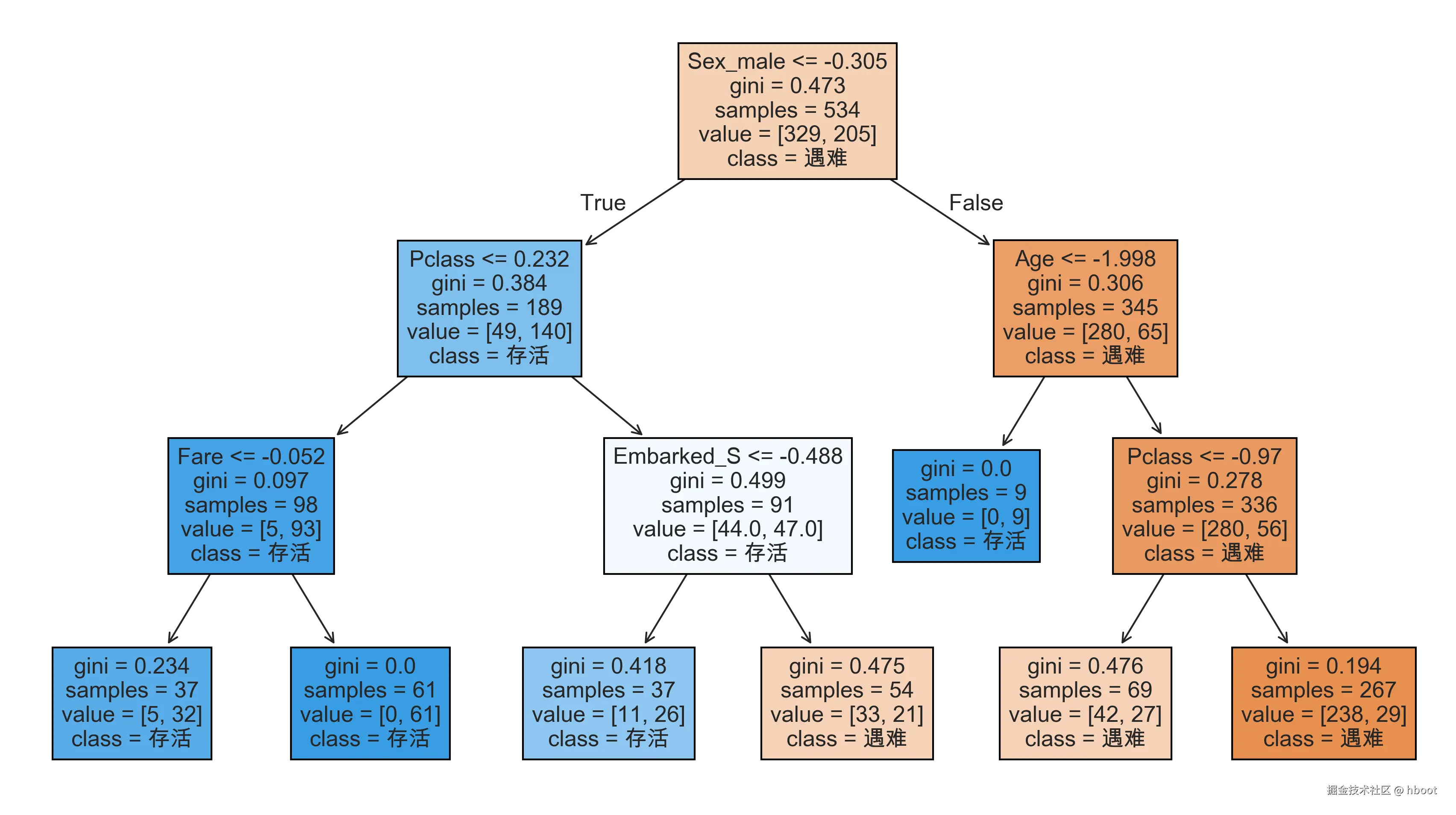
决策树节点属性说明:
- 决策条件,比如性别、年龄等。
gini基尼指数,越小越纯samples样本数量value节点结果数量class节点结果
随机森林
用途: 多棵决策树投票,效果更稳定
原理: 训练多棵不同的决策树,取多数投票结果
js
决策树1 → 存活
决策树2 → 遇难
决策树3 → 存活
决策树4 → 存活
决策树5 → 遇难
─────────────────
最终结果 → 存活(3:2)
py
from sklearn.ensemble import RandomForestClassifier

model = RandomForestClassifier(n_estimators=100, random_state=42)
model.fit(X_train, y_train)  # 树模型不需要缩放

# 特征重要性
importance = pd.Series(model.feature_importances_, index=X.columns)
importance.sort_values(ascending=False).plot(kind="bar")
plt.title("特征重要性")
plt.show()
特征重要性: 每个特征对预测结果的影响,越大越重要。
K-Means 聚类
用途: 无监督学习,自动把数据分成 K 组。使用场景:聚类、图像处理、广告推荐、推荐引擎、 anomaly detection(异常检测)
原理: 不断调整 K 个中心点,让每个点到最近中心点的距离最小
js
步骤1:随机放 K 个中心点
步骤2:每个点归到最近的中心点
步骤3:重新计算中心点位置
步骤4:重复 2-3 直到不再变化
py
from sklearn.cluster import KMeans

# 全量缩放
scaler = StandardScaler()
X_scaled = scaler.fit_transform(X)

# 创建模型
model = KMeans(n_clusters=3, random_state=42)
model.fit(X_scaled)

# 获取聚类结果
labels = model.labels_        # 每个点属于哪个簇
centers = model.cluster_centers_  # 中心点坐标

# 可视化
plt.scatter(X_scaled[:, 0], X_scaled[:, 1], c=labels, cmap="viridis")
plt.scatter(centers[:, 0], centers[:, 1], c="red", marker="x", s=200)
plt.title("K-Means 聚类结果")
plt.show()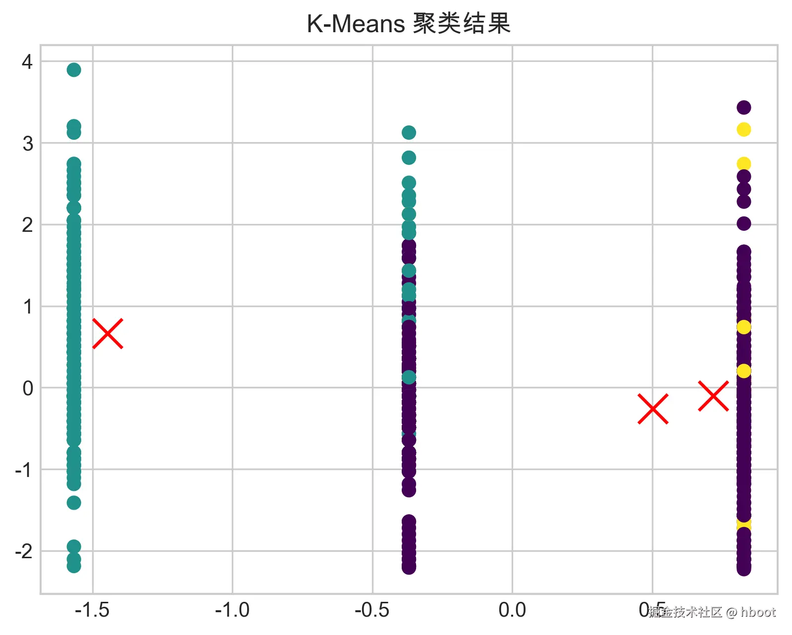
K-Means 聚类结果: 每个点属于哪个簇,以及中心点坐标。对于如何分组,需要不断尝试最优的k。只能发现球形聚类,不能发现长条形、环形分区。受异常数据影响较大。
实战:Titanic 存活预测
在上一章【AI工程师第二课 - 数据处理】中对于数据的清理分析做了详细的阐述,这里重点完成kaggle的任务,通过真实的Titanic 存活数据训练模型,然后得出测试数据的存活预测。
前面的章节已经部分包含了所需要的代码逻辑,这里按照流程给出全部的代码。
1. 数据加载与清洗
py
import pandas as pd

df = pd.read_csv("train.csv")

# 特征选择
features = ["Pclass", "Sex", "Age", "SibSp", "Parch", "Fare", "Embarked"]
df = df[features + ["Survived"]]

# 缺失值处理
df["Age"] = df["Age"].fillna(df["Age"].median())
df["Embarked"] = df["Embarked"].fillna(df["Embarked"].mode()[0])

# 类别编码
df["Sex"] = df["Sex"].map({"female": 0, "male": 1})
df = pd.get_dummies(df, columns=["Embarked"], drop_first=True)
2. 特征工程:划分数据集/特征缩放
这里只划分了训练集和测试集,没有划分验证集。因为总数据量少,后面使用了交叉验证代替了固定划分,让更多的数据参与训练,提高水利用率。
py
X = df.drop("Survived", axis=1)
y = df["Survived"]

# 划分数据集
X_train, X_test, y_train, y_test = train_test_split(
    X, y, test_size=0.2, random_state=42
)

# 特征缩放
scaler = StandardScaler()
X_train_scaled = scaler.fit_transform(X_train)
X_test_scaled = scaler.transform(X_test)
3. 模型训练与评估
是否存活就是典型的二分类问题,使用逻辑回归和随机森林模型训练和评估。
py
from sklearn.linear_model import LogisticRegression
from sklearn.ensemble import RandomForestClassifier

# 模型1:逻辑回归
lr = LogisticRegression(max_iter=1000)
lr.fit(X_train_scaled, y_train)
lr_score = lr.score(X_test_scaled, y_test)
print(f"\n逻辑回归准确率:{lr_score:.3f}")

# 模型2:随机森林
rf = RandomForestClassifier(n_estimators=100, random_state=42)
rf.fit(X_train, y_train)  # 随机森林不需要缩放
rf_score = rf.score(X_test, y_test)
print(f"随机森林准确率:{rf_score:.3f}")
没想到两个测试集的准确率都是0.81,说明模型效果都不错。
4. 交叉验证
py
from sklearn.model_selection import cross_val_score

# 交叉验证
lr_cv = cross_val_score(lr, X_train_scaled, y_train, cv=5)
rf_cv = cross_val_score(rf, X_train, y_train, cv=5)

print(f"\n逻辑回归 5折交叉验证:{lr_cv.mean():.3f} ± {lr_cv.std():.3f}")
print(f"随机森林 5折交叉验证:{rf_cv.mean():.3f} ± {rf_cv.std():.3f}")
交叉验证的结果随机森林的准确率更高一点,而且误差更小,说明随机森林效果更好。
5. 详细评估
我们已经知道了随机森林的预测效果更好,下面详细评估。
py
best_model = rf
y_pred = best_model.predict(X_test)

print("\n=== 混淆矩阵 ===")
print(confusion_matrix(y_test, y_pred))

print("\n=== 分类报告 ===")
print(classification_report(y_test, y_pred, target_names=["遇难", "存活"]))
结果输出:
js
=== 混淆矩阵 ===
[[90 15]        ← 105 个遇难:90 对,15 错
 [19 55]]       ← 74 个存活:55 对,19 错

=== 分类报告 ===
              precision    recall  f1-score   support

        遇难       0.83      0.86      0.84       105
        存活       0.79      0.74      0.76        74

    accuracy                           0.81       179
   macro avg       0.81      0.80      0.80       179
weighted avg       0.81      0.81      0.81       179
6. 特征重要性
py
importance = pd.Series(best_model.feature_importances_, index=X.columns)
importance.sort_values(ascending=True).plot(kind="barh")
plt.title("特征重要性")
plt.xlabel("重要性")
plt.tight_layout()
plt.show()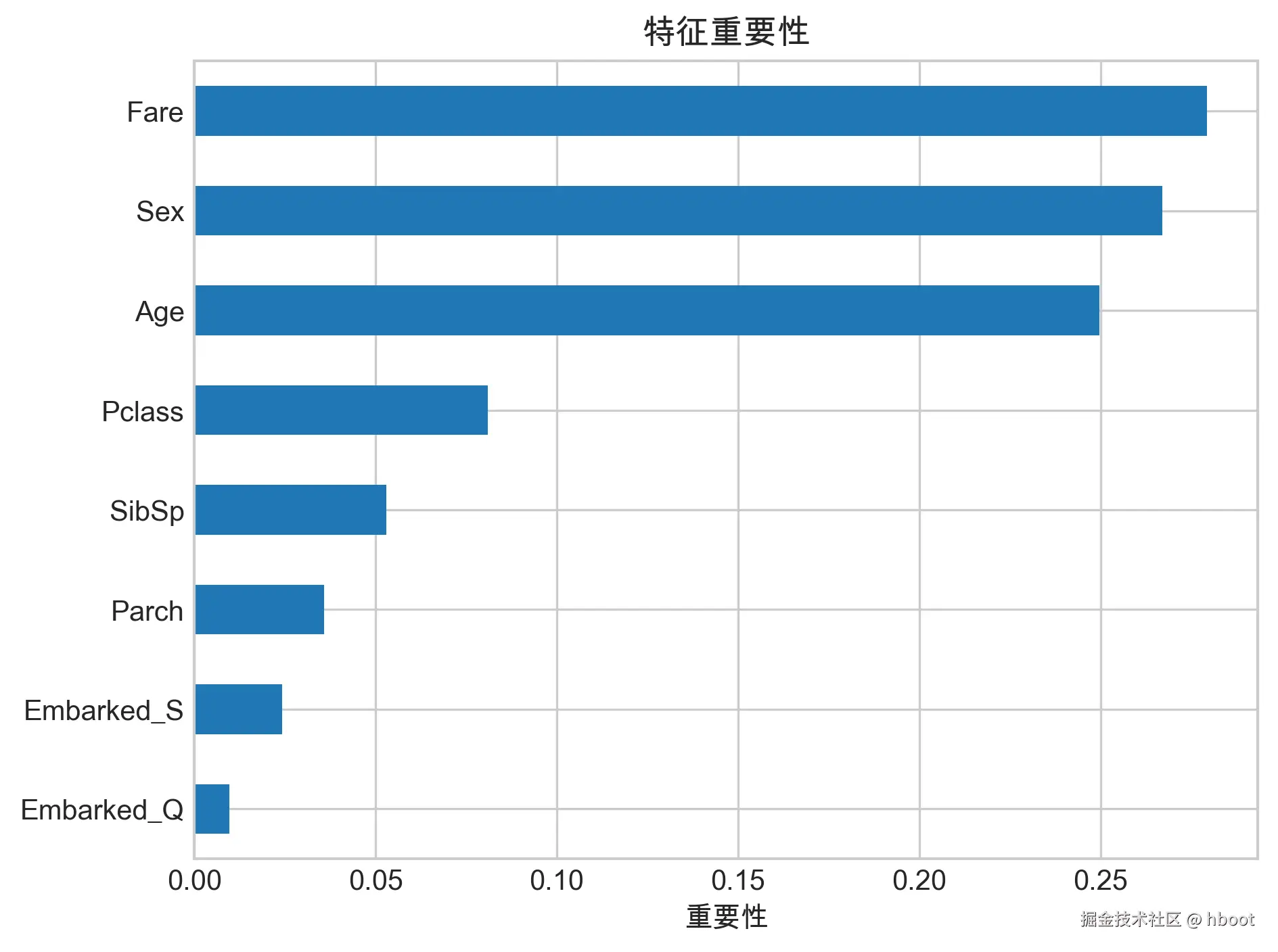
7. 预测测试集
py
# 加载测试数据集
test_df = pd.read_csv("test.csv")
passenger_ids = test_df["PassengerId"]

# 用同样的特征
test_df = test_df[features]

# 清洗数据
test_df["Age"] = test_df["Age"].fillna(test_df["Age"].median())
test_df["Fare"] = test_df["Fare"].fillna(test_df["Fare"].median())
test_df["Embarked"] = test_df["Embarked"].fillna(test_df["Embarked"].mode()[0])

# 类别编码
test_df["Sex"] = test_df["Sex"].map({"female": 0, "male": 1})
test_df = pd.get_dummies(test_df, columns=["Embarked"], drop_first=True)


# 预测
predictions = best_model.predict(test_df)

# 生成提交文件
submission = pd.DataFrame({
    "PassengerId": passenger_ids,
    "Survived": predictions
})
submission.to_csv("submission.csv", index=False)
print("提交文件已生成!")
得到测试集的预测结果,我们可以提交结果到kaggle进行评价。
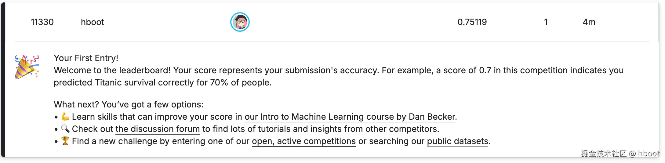
可以看到结果分数为0.75, 排行榜排名11330。还有比我们低的,🤣 。
8. 优化
- 通过构造新特征来提升模型效果。比如:提取称谓(女士可能存活率高)、家庭人数。
- 换更好的模型。比如:KNN、SVM、XGBoost、LightGBM。
- 调参。
- 集成模型。多个模型投票,取最终结果。
我们先通过调参来试试能提升多少。GridSearchCV 可以自动搜索参数,找到最佳参数组合。
py
from sklearn.model_selection import GridSearchCV

# 定义参数网格
params = {
    "n_estimators": [50, 100, 200], # 树数量
    "max_depth": [3, 5, 10, None], # 树深度
    "min_samples_split": [2, 5, 10], # 节点分裂所需的最小样本数
    "min_samples_leaf": [1, 2, 4], # 节点叶子所需最小样本数
}

# 网格搜索
grid = GridSearchCV(
    RandomForestClassifier(random_state=42),
    params,
    cv=5, # 交叉验证次数
    scoring="accuracy", # 评估标准
    n_jobs=-1  # 用所有 CPU 核心,加快速度
)

# 3 x 3 x 4 x 3 = 108 个参数组合 + 5 个交叉验证,共 108 x 5 = 540 个模型训练
grid.fit(X_train, y_train)

print(f"最优参数:{grid.best_params_}")
print(f"最优分数:{grid.best_score_:.3f}")

best_rf = grid.best_estimator_
predictions = best_rf.predict(test_df)

# 生成提交文件
submission = pd.DataFrame({
    "PassengerId": passenger_ids,
    "Survived": predictions
})
submission.to_csv("submission_optimized.csv", index=False)
print("提交文件已生成!")再次提交查看结果排名,可以看到分数从0.75提升到0.78,虽然看似提升不大, 但还是能提升。而且排名飙升到了2513,可以想像0.01分之要甩掉多少人。

算法选择指南
| 任务类型 | 数据特点 | 推荐算法 | 理由 |
|---|---|---|---|
| 二分类 | 数据量小 | 逻辑回归 | 简单、可解释 |
| 二分类 | 数据量大 | 随机森林 | 效果好、不易过拟合 |
| 回归 | 线性关系 | 线性回归 | 简单、可解释 |
| 回归 | 非线性关系 | 随机森林 | 能捕捉复杂关系 |
| 聚类 | 不知道分几组 | K-Means | 最常用 |
一句话:先跑逻辑回归做 baseline,再用随机森林提升效果。
常见坑
| 坑 | 说明 | 解决 |
|---|---|---|
| 数据泄露 | 测试集信息混入训练集 | 用 train_test_split 后再做特征工程 |
| 特征缩放 | 树模型不需要,线性模型需要 | 随机森林不缩放,逻辑回归要缩放 |
| 类别不平衡 | 正负样本比例悬殊 | 用 class_weight="balanced" |
| 过拟合 | 训练集表现远好于测试集 | 交叉验证、限制模型复杂度 |