CSDN博客-第5天-PyTorch标准训练流程与XOR

【深度学习入门 Day 5】PyTorch 标准训练流程：用 nn.Module 训练 XOR

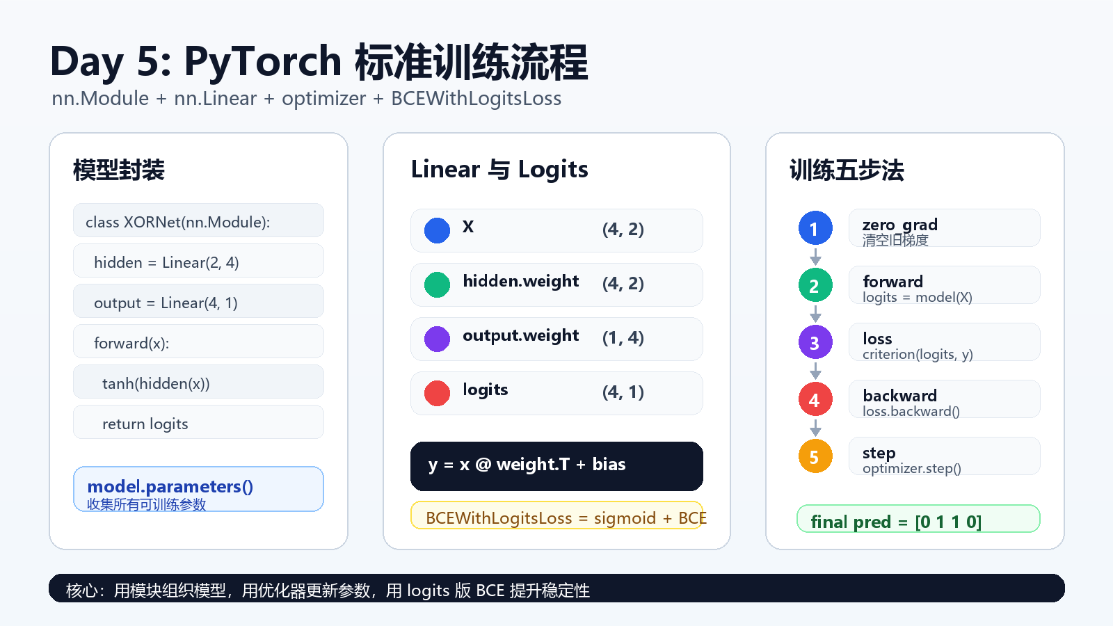
本文记录深度学习学习第 5 天的内容：把昨天"手动创建参数 + 手动更新参数"的 PyTorch XOR 程序，改写成更标准的 PyTorch 工程写法。今天重点理解 nn.Module、nn.Linear、model.parameters()、optimizer、标准训练循环，以及为什么二分类任务更推荐使用 BCEWithLogitsLoss。

文章目录

• 一、从手动 PyTorch 到标准 PyTorch
• 二、准备 XOR 数据
• 三、用 nn.Module 封装模型
• 四、理解 nn.Linear 的参数形状
• 五、前向传播：model(X) 背后发生了什么
• 六、损失函数：为什么推荐 BCEWithLogitsLoss
• 七、优化器：用 optimizer 管理参数更新
• 八、标准训练循环五步法
• 九、完整训练代码
• 十、运行结果
• 十一、今日总结
• 十二、课后自测

---

一、从手动 PyTorch 到标准 PyTorch

昨天我们已经用 PyTorch 自动求导训练了 XOR，但参数还是手动管理的：

W1 = (torch.randn(2, 4) * 0.1).requires_grad_()
b1 = torch.zeros(1, 4, requires_grad=True)

W2 = (torch.randn(4, 1) * 0.1).requires_grad_()
b2 = torch.zeros(1, 1, requires_grad=True)

更新参数时也手动写：

with torch.no_grad():
    W1 -= lr * W1.grad
    b1 -= lr * b1.grad
    W2 -= lr * W2.grad
    b2 -= lr * b2.grad

这对理解自动求导非常有帮助，但在真实项目里，我们更常用 PyTorch 标准写法：

nn.Module       封装模型
nn.Linear       自动创建线性层参数
loss.backward() 自动计算梯度
optimizer.step() 自动更新参数

今天的目标是把 XOR 模型写成更正式的训练脚本。

---

二、准备 XOR 数据

先准备数据：

import torch
import torch.nn as nn


def build_xor_data():
    X = torch.tensor([
        [0.0, 0.0],
        [0.0, 1.0],
        [1.0, 0.0],
        [1.0, 1.0],
    ])

    y = torch.tensor([
        [0.0],
        [1.0],
        [1.0],
        [0.0],
    ])

    return X, y

XOR 的目标仍然是：

[0, 0] -> 0
[0, 1] -> 1
[1, 0] -> 1
[1, 1] -> 0

形状是：

X.shape = (4, 2)
y.shape = (4, 1)

含义：

4 个样本
每个样本 2 个特征
每个样本 1 个二分类标签

---

三、用 nn.Module 封装模型

今天不再手动写 W1, b1, W2, b2，而是定义一个模型类：

class XORNet(nn.Module):
    def __init__(self):
        super().__init__()
        self.hidden = nn.Linear(2, 4)
        self.output = nn.Linear(4, 1)

    def forward(self, x):
        x = torch.tanh(self.hidden(x))
        logits = self.output(x)
        return logits

逐行理解。

class XORNet(nn.Module):

表示 XORNet 是一个 PyTorch 模型。

super().__init__()

表示先初始化 nn.Module 这个基类。这样 PyTorch 才能正确管理模型里的参数、子模块和训练状态。

self.hidden = nn.Linear(2, 4)

表示第一层线性层：

输入 2 维
输出 4 维

self.output = nn.Linear(4, 1)

表示第二层线性层：

输入 4 维
输出 1 维

def forward(self, x):

定义前向传播逻辑。

以后调用：

logits = model(X)

PyTorch 实际会调用：

model.forward(X)

---

四、理解 nn.Linear 的参数形状

实例化模型：

torch.manual_seed(42)

model = XORNet()
print(model)

输出：

XORNet(
  (hidden): Linear(in_features=2, out_features=4, bias=True)
  (output): Linear(in_features=4, out_features=1, bias=True)
)

再打印参数：

for name, param in model.named_parameters():
    print(name, param.shape)

输出：

hidden.weight torch.Size([4, 2])
hidden.bias torch.Size([4])
output.weight torch.Size([1, 4])
output.bias torch.Size([1])

这里有一个重要细节。

我们手写 NumPy/PyTorch 时，第一层参数常写成：

W1.shape = (2, 4)

因为：

X @ W1 = (4, 2) @ (2, 4) = (4, 4)

但 PyTorch 的 nn.Linear(2, 4) 内部保存的是：

weight.shape = (out_features, in_features) = (4, 2)

它内部计算是：

y = x @ weight.T + bias

所以：

X.shape             = (4, 2)
hidden.weight.shape = (4, 2)
hidden.weight.T     = (2, 4)

X @ hidden.weight.T = (4, 2) @ (2, 4) = (4, 4)

从用户角度看，只需要记住：

nn.Linear(in_features, out_features)

也就是：

nn.Linear(2, 4)

表示"输入 2 维，输出 4 维"。

---

五、前向传播：model(X) 背后发生了什么

做一次前向传播：

logits = model(X)

它等价于执行：

x = torch.tanh(model.hidden(X))
logits = model.output(x)

注意今天的模型输出叫 logits，而不是概率。

logits = 模型输出的原始分数
prob = sigmoid(logits) 后得到的概率

也就是说：

prob = torch.sigmoid(logits)

才是属于 1 类的概率。

为什么今天不在 forward() 里写 sigmoid？

因为我们要使用更稳定的损失函数：

nn.BCEWithLogitsLoss()

它内部会自动完成：

sigmoid + BCE

---

六、损失函数：为什么推荐 BCEWithLogitsLoss

昨天的写法是：

模型输出概率 a2
损失函数用 BCELoss

也就是：

x = torch.sigmoid(self.output(x))
criterion = nn.BCELoss()

今天更推荐：

模型输出 logits
损失函数用 BCEWithLogitsLoss

也就是：

logits = self.output(x)
criterion = nn.BCEWithLogitsLoss()

BCEWithLogitsLoss 可以理解成：

BCEWithLogitsLoss = sigmoid + BCELoss 的数值稳定合并版

它的好处是：

1. 不需要在模型最后手动写 sigmoid。
2. 内部计算更稳定。
3. 当输出分数很大或很小时，更不容易出现数值问题。

对于 XOR 这种小实验，两种写法都可以训练成功。但对于真实二分类任务，更推荐：

criterion = nn.BCEWithLogitsLoss()

预测时再单独做：

prob = torch.sigmoid(logits)
pred = (prob >= 0.5).int()

---

七、优化器：用 optimizer 管理参数更新

昨天手动更新参数：

with torch.no_grad():
    W1 -= lr * W1.grad
    b1 -= lr * b1.grad
    W2 -= lr * W2.grad
    b2 -= lr * b2.grad

今天交给优化器：

optimizer = torch.optim.SGD(model.parameters(), lr=0.1)

这里：

model.parameters()

会把模型里所有需要训练的参数交给优化器，包括：

hidden.weight
hidden.bias
output.weight
output.bias

之后只要调用：

optimizer.step()

优化器就会根据这些参数的 .grad 自动更新参数。

也就是说：

手动更新 W、b

变成了：

optimizer 管理所有参数更新

---

八、标准训练循环五步法

PyTorch 的标准训练循环可以压缩成 5 步：

optimizer.zero_grad()

logits = model(X)
loss = criterion(logits, y)

loss.backward()
optimizer.step()

逐行理解：

optimizer.zero_grad()

清空上一轮梯度。因为 PyTorch 的梯度默认会累加。

logits = model(X)

前向传播，得到模型输出。

loss = criterion(logits, y)

计算损失。

loss.backward()

自动反向传播，把梯度保存到各个参数的 .grad 中。

optimizer.step()

根据梯度更新模型参数。

以后训练 CNN、RNN、Transformer，本质上还是这个骨架，只是：

model 更复杂
data 更大
loss 可能不同
optimizer 可能换成 Adam

---

九、完整训练代码

import torch
import torch.nn as nn


def build_xor_data():
    X = torch.tensor([
        [0.0, 0.0],
        [0.0, 1.0],
        [1.0, 0.0],
        [1.0, 1.0],
    ])

    y = torch.tensor([
        [0.0],
        [1.0],
        [1.0],
        [0.0],
    ])

    return X, y


class XORNet(nn.Module):
    def __init__(self):
        super().__init__()
        self.hidden = nn.Linear(2, 4)
        self.output = nn.Linear(4, 1)

    def forward(self, x):
        x = torch.tanh(self.hidden(x))
        logits = self.output(x)
        return logits


def print_model_info(model):
    print(model)
    print("\nparameters:")
    for name, param in model.named_parameters():
        print(f"{name:14s} {tuple(param.shape)}")


def train(model, X, y, epochs=10001, lr=0.1):
    criterion = nn.BCEWithLogitsLoss()
    optimizer = torch.optim.SGD(model.parameters(), lr=lr)

    for step in range(epochs):
        optimizer.zero_grad()

        logits = model(X)
        loss = criterion(logits, y)

        loss.backward()
        optimizer.step()

        if step % 1000 == 0:
            with torch.no_grad():
                prob = torch.sigmoid(logits)
                pred = (prob >= 0.5).int()

            print(
                f"step={step:05d}, "
                f"loss={loss.item():.6f}, "
                f"prob={prob.view(-1).numpy().round(3)}, "
                f"pred={pred.view(-1).numpy()}"
            )


def evaluate(model, X, y):
    with torch.no_grad():
        logits = model(X)
        prob = torch.sigmoid(logits)
        pred = (prob >= 0.5).int()

    print("\nfinal result:")
    print("prob:", prob.view(-1).numpy().round(4))
    print("pred:", pred.view(-1).numpy())
    print("true:", y.view(-1).int().numpy())


def main():
    torch.manual_seed(42)

    X, y = build_xor_data()
    model = XORNet()

    print("X shape:", tuple(X.shape))
    print("y shape:", tuple(y.shape))
    print_model_info(model)

    train(model, X, y)
    evaluate(model, X, y)


if __name__ == "__main__":
    main()

---

十、运行结果

运行后可以看到：

X shape: (4, 2)
y shape: (4, 1)
XORNet(
  (hidden): Linear(in_features=2, out_features=4, bias=True)
  (output): Linear(in_features=4, out_features=1, bias=True)
)

parameters:
hidden.weight  (4, 2)
hidden.bias    (4,)
output.weight  (1, 4)
output.bias    (1,)

训练过程：

step=00000, loss=0.759778, prob=[0.664 0.695 0.683 0.7  ], pred=[1 1 1 1]
step=01000, loss=0.051991, prob=[0.016 0.945 0.942 0.073], pred=[0 1 1 0]
step=02000, loss=0.016744, prob=[0.004 0.981 0.981 0.024], pred=[0 1 1 0]
...
step=10000, loss=0.002075, prob=[0.001 0.998 0.998 0.003], pred=[0 1 1 0]

最终结果：

final result:
prob: [0.0005 0.9976 0.9976 0.003 ]
pred: [0 1 1 0]
true: [0 1 1 0]

说明模型已经成功学会 XOR。

---

十一、今日总结

今天的核心内容可以压缩成 6 点：

1. nn.Module 用来封装模型结构和参数。
2. nn.Linear(in_features, out_features) 自动创建线性层的权重和偏置。
3. PyTorch 的 Linear.weight 形状是 (out_features, in_features)。
4. model.parameters() 会收集模型中所有需要训练的参数。
5. optimizer.zero_grad() -> forward -> loss -> backward -> optimizer.step() 是 PyTorch 标准训练骨架。
6. 二分类任务更推荐 BCEWithLogitsLoss，模型输出 logits，预测时再手动 sigmoid。

最终要记住这句话：

Day4 学的是 PyTorch 如何自动求导，Day5 学的是 PyTorch 如何用标准模块组织一次完整训练。

---

十二、课后自测

1. nn.Module 的作用是什么？
2. 为什么要在 __init__() 里写 super().__init__()？
3. nn.Linear(2, 4) 表示什么？
4. 为什么 hidden.weight.shape 是 (4, 2)，而不是 (2, 4)？
5. model.parameters() 返回的是什么？
6. optimizer.zero_grad() 为什么要放在每轮训练开始？
7. optimizer.step() 做了什么？
8. 为什么二分类任务推荐 BCEWithLogitsLoss？
9. 使用 BCEWithLogitsLoss 时，模型最后一层还需要手动写 sigmoid 吗？
10. 预测时为什么还要对 logits 调用 torch.sigmoid()？