结构大体是
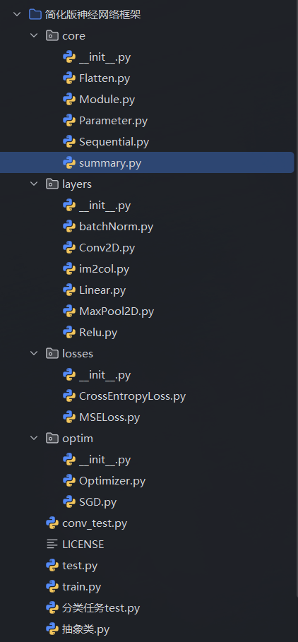
github:https://github.com/helloworldzzx/MiniML
一、Module.py
为什么所有层都要继承 Module?
因为神经网络希望把所有层当成"同一种东西"。
例如:
输入
 ↓
Linear
 ↓
ReLU
 ↓
Linear
 ↓
Softmax
如果每层长得都不一样:
Linear.compute()

Conv.run()

ReLU.work()
那 Sequential 根本不知道该调用谁。
所以必须统一接口。
所有层都必须有:
python
forward()
backward()
这就是面向对象的多态(Polymorphism)。
Module保存什么
- 规定接口,让所有层必须支持,比如都要有
forward、backward - 管理参数,
例如:
Linear有:W b
Conv有:Kernel Bias
Relu没有参数
那么layer.parameters()对于不同层返回不同的东西
Optimizer 根本不用关心是什么层。它只需要:
python
for p in model.parameters():
更新- 方便组合
python
Sequential(
    Linear(),
    ReLU(),
    Linear()
)
实际上就是一个Module,里面放很多Module
以后Sequential.forward()里面再调用 Linear.forward() ReLU.forward() Linear.forward()
这就是 PyTorch 的设计。
python
from abc import ABC, abstractmethod
#ABC:抽象基类父类,自定义抽象类必须继承它
#abstractmethod:装饰器,标记方法为抽象方法,只有声明,没有实现逻辑
#子类继承并必须实现全部抽象方法
class Module(ABC):
    """
    所有网络层的父类。
    每一个层(Linear、Conv、ReLU......)
    都必须继承 Module。

    子类需要实现:
        forward()
        backward()

    如果该层有参数(例如 Linear、Conv),
    还需要返回参数列表。
    """

    @abstractmethod
    def forward(self, x):
        """
        前向传播
        输入:x(ndarray)
        输出:当前层的输出
        """
        pass

    @abstractmethod
    def backward(self, grad_output):
        """
        反向传播

        输入:grad_output(loss对当前层输出的梯度)
        输出:loss对当前层输入的梯度
        """
        pass

    def parameters(self):
        """
        返回需要训练的参数。

        比如:ReLU没有参数,默认返回空列表。
             Linear、Conv需要重写这个函数。
        """
        return []
二、Parameter
在cs231n中,Linear写法如下:
python
class Linear(Module):
    def __init__(self, in_features, out_features):
        self.W = np.random.randn(in_features, out_features)
        self.b = np.zeros(out_features)
        self.dW = np.zeros_like(self.W)
        self.db = np.zeros_like(self.b)
这种写法有缺点:
W和dW应该是一个对象的两个属性,而且后面还有不同的其他要求梯度,表示起来很麻烦,这时候就要封装一下:
一个对象
↓
里面有
data
grad

比如:
weight.data
weight.grad
python
import numpy as np


class Parameter:
    """
    神经网络中的可训练参数。
    每个参数都包含:
        data : 参数值
        grad : 参数梯度
    """

    def __init__(self, data):
        """
        初始值data : ndarray
        """
        self.data = data

        # 梯度初始化为0
        self.grad = np.zeros_like(data)

    def zero_grad(self):
        """
        梯度清零。
        每次反向传播之前调用。
        """
        self.grad.fill(0)
三、Linear
- init
py
def __init__(self, in_features, out_features):形参是输入层和输出层神经元数量
比如: layer = Linear(10,5)代表输入层是10个维度(接受样本的10个指标),输出层5个维度
- weight初始化
py
weight = np.random.randn(
    in_features,
    out_features
)
weight的形状等于Linear的参数
这里使用正态分布随机数,不使用0填充,因为如果所有神经元的权重一样,那么:
Forward
全部输出一样。
Backward
梯度也一样。
以后:
永远一样。
神经元就没有分工了。
-
bias初始化
bias的形状等于weight的第二个参数,因为第二个表示神经元个数,每个神经元一个bias。可以初始化为0
-
forward和backward
假设只有两个输入:
x₁ = 2
x₂ = 3
一个神经元:
w₁ = 0.5
w₂ = 1.2
b = 1
网络结构:
x1 -----\
         \
           >(+b) 神经元 ----> y
         /
x2 -----/
y = x 1 w 1 + x 2 w 2 + b y=x_1w_1+x_2w_2+b y=x1w1+x2w2+b
代入数字:
y = 2×0.5 + 3×1.2 +1
  =1+3.6+1
  =5.6
这就是forward
然后引入Loss
假设真实值t=6
使用平方误差:
L = 1 2 ( y − t ) 2 L=\frac{1}{2}(y-t)^2 L=21(y−t)2
得到
L=1/2 × (5.6-6)^2=0.08Forward 全结束。
然后开始Backward
现在我们希望
调整w₁、w₂、b,让Loss变小
那么首先求
∂ L ∂ y \frac{\partial L}{\partial y} ∂y∂L
根据链式法则:
L = 1 2 ( y − t ) 2 L=\frac{1}{2}(y-t)^2 L=21(y−t)2
求导:
∂ L ∂ y = y − t \frac{\partial L}{\partial y}=y-t ∂y∂L=y−t
得到:
dout = 5.6 - 6 = -0.4这就是代码中的grad_output
它不是凭空来的,而是上一层(Loss)传下来的梯度。
然后求 W 1 W_1 W1的梯度
因为 y = x 1 w 1 + x 2 w 2 + b y=x_1w_1+x_2w_2+b y=x1w1+x2w2+b
所以
∂ L ∂ w 1 = ∂ L ∂ y ⋅ ∂ y ∂ w 1 \frac{\partial L}{\partial w_1} = \frac{\partial L}{\partial y}\cdot \frac{\partial y}{\partial w_1} ∂w1∂L=∂y∂L⋅∂w1∂y
前面已经知道了 ∂ L ∂ y = − 0.4 \frac{\partial L}{\partial y}=-0.4 ∂y∂L=−0.4,而 ∂ y ∂ w 1 = x 1 \frac{\partial y}{\partial w_1}=x_1 ∂w1∂y=x1,所以 ∂ L ∂ w 1 = − 0.4 × 2 = − 0.8 \frac{\partial L}{\partial w_1}=-0.4 \times 2 = -0.8 ∂w1∂L=−0.4×2=−0.8
同理 ∂ L ∂ w 2 = − 0.4 × 3 = − 1.2 \frac{\partial L}{\partial w_2}=-0.4 \times 3 = -1.2 ∂w2∂L=−0.4×3=−1.2
bias
∂ y ∂ b = 1 \frac{\partial y}{\partial b} = 1 ∂b∂y=1
所以
∂ L ∂ b = − 0.4 \frac{\partial L}{\partial b} = -0.4 ∂b∂L=−0.4
所以得到规律
对于一个神经元
dw = x × dout对于多个神经元
例如:输入2维,输出3个神经元
      y1  y2  y3

x1    w11 w12 w13

x2    w21 w22 w23
w = 2 × 3
y 1 = x 1 w 11 + x 2 w 21 y 2 = x 1 w 12 + x 2 w 22 y 3 = x 1 w 13 + x 2 w 23 d o u t = ∂ L ∂ y = y − y i y_1 = x_1w_{11}+x_2w_{21} \\ y_2 = x_1w_{12}+x_2w_{22}\\ y_3 = x_1w_{13}+x_2w_{23}\\ dout=\frac{\partial L}{\partial y}=y-y_i y1=x1w11+x2w21y2=x1w12+x2w22y3=x1w13+x2w23dout=∂y∂L=y−yi
现在:
Loss 会给三个梯度:
dout
=
[
dy1
dy2
dy3
]
对于神经元:
dw11=x1×dy1
dw12=x1×dy2
dw13=x1×dy3
dw21=x2×dy1
dw22=x2×dy2
dw23=x2×dy3
整理发现:
        dy1  dy2  dy3

x1

x2
这是一个矩阵了,其实就是:
输入ᵀ
×
输出梯度
也就是:
d W = x T d o u t dW = x^T dout dW=xTdout
下面介绍Batch
真正的训练时,不是1个样本,而是例如32个样本,假设样本有10个维度,则输入
x.shape=(32,10)先看一个样本
	y1	y2	y3	y4	y5
x1	w11	w12	w13	w14	w15
x2	w21	w22	w23	w24	w25
x3	...
x4
x5
x6
x7
x8
x9
x10

可视化
x1 -----\
x2 ----- \
x3 -----  \
x4 -----   \
x5 -----     > 神经元 ----> yi----->Loss
x6 -----    /
x7 -----   /
x8 -----  /
x9 ----- /
x10 ----/
一个样本有5个dout(对应5个神经元),32个样本就是dout(32,5)
权重w(10,5)5个神经元,每个神经元有10个权重参数,接收10个维度
X.T(10,32) × dout(32,5) = (10,5)
python
self.W.grad = self.x.T @ grad_output至此dw已经得到,
然后求dx同理
要求:
∂ L ∂ X \frac{\partial L}{\partial X} ∂X∂L
由于 Y = X W + b Y=XW + b Y=XW+b
展开看:
例如
y 1 = x 1 w 11 + x 2 w 21 + . . . y 2 = x 1 w 12 + x 2 w 22 + . . . y 3 = x 1 w 13 + x 2 w 23 + . . . . . . y_1=x_1w_{11}+x_2w_{21}+...\\ y_2=x_1w_{12}+x_2w_{22}+...\\ y_3=x_1w_{13}+x_2w_{23}+...\\ ... y1=x1w11+x2w21+...y2=x1w12+x2w22+...y3=x1w13+x2w23+......
对于输入x1,它会影响所有的输出神经元:
x1		x1		x1 		...
↓		↓		↓
y1		y2		y3
↓		↓		↓
Loss	Loss	Loss
所以
∂ L ∂ x 1 = ∑ j ∂ L ∂ y i ∂ y i ∂ x 1 \frac{\partial L}{\partial x_1}=\sum_{j}^{}\frac{\partial L}{\partial y_i}\frac{\partial y_i}{\partial x_1} ∂x1∂L=j∑∂yi∂L∂x1∂yi
其中 ∂ y i ∂ x i = w i j \frac{\partial y_i}{\partial x_i}=w_{ij} ∂xi∂yi=wij
整理成矩阵:
d X = d o u t ⋅ W T dX=dout \cdot W^T dX=dout⋅WT
py
dx = grad_output @ self.W.data.Tdb比较简单推导
比如
y = x 1 w 1 + x 2 w 2 + b y=x_1w_1+x_2w_2+b y=x1w1+x2w2+b
要求:
∂ L ∂ b \frac{\partial L}{\partial b} ∂b∂L
链式法则:
∂ L ∂ b = ∂ L ∂ y ⋅ ∂ y ∂ b \frac{\partial L}{\partial b}=\frac{\partial L}{\partial y}\cdot \frac{\partial y}{\partial b} ∂b∂L=∂y∂L⋅∂b∂y
其中 ∂ L ∂ y = d o u t \frac{\partial L}{\partial y}=dout ∂y∂L=dout, ∂ y ∂ b = 1 \frac{\partial y}{\partial b}=1 ∂b∂y=1
所以
∂ L ∂ b = d o u t \frac{\partial L}{\partial b}=dout ∂b∂L=dout
扩展到多个神经元
b=[b1,b2,b3]
y1=xW+b1
y2=xW+b2
y3=xW+b3
每个bias的梯度:
db_1 = dout_1\\ db_2 = dout_2\\ db_3 = dout_3 db = dout
py
self.b.grad = np.sum(
    grad_output,
    axis=0
)
为什么不是直接等于 grad_output?
因为我们现在不是一个样本,而是一个 Batch。
比如grad_output.shape=(32,5)
表示32个样本,每个有5个输出神经元
例如:
sample1

[-0.2  0.5  1.0  0.3  -0.8]

sample2

[ 0.1 -0.4  0.2  0.5   0.7]

...

sample32
注意:
这 32 个样本共用同一组 bias!
所以对于:
b1
它收到的梯度应该是:
sample1贡献

+

sample2贡献

+

...

+

sample32贡献
所以
d b = ∑ i = 1 N d o u t i db=\sum_{i=1}^{N}dout_i db=i=1∑Ndouti
N为batchSize,douti为第i个样本对bias的梯度
py
import numpy as np

from core.Module import Module
from core.Parameter import Parameter


class Linear(Module):
    """
    全连接层
    Y = XW + b
    X : (N, in_features)
    W : (in_features, out_features)
    b : (out_features,)
    Y : (N, out_features)
    """

    def __init__(self, in_features, out_features):

        # He初始化
        weight = np.random.randn(
            in_features,
            out_features
        ) * np.sqrt(2.0 / in_features)

        #Xavier初始化,正态分布
        # weight = np.random.randn(
        #     in_features,
        #     out_features
        # ) * np.sqrt(
        #     2.0 / (in_features * out_features)
        # )

        #Xavier初始化,均匀分布
        # limit = np.sqrt(2.0 / (in_features + out_features))
        # weight = np.random.uniform(
        #     -limit,
        #     limit,
        #     size=(in_features, out_features)
        # )

        bias = np.zeros(out_features)

        self.W = Parameter(weight)

        self.b = Parameter(bias)

        # forward时缓存输入
        self.x = None

    def forward(self, x):

        """
        x.shape
        (batch_size, in_features)
        例如:
        (32,10)
        """

        self.x = x

        out = x @ self.W.data + self.b.data

        return out

    def backward(self, grad_output):

        """
        grad_output
        dL/dY
        shape:
        (batch_size, out_features)
        例如:
        (32,5)
        """

        # (10,32) @ (32,5)
        # = (10,5)

        self.W.grad = self.x.T @ grad_output

        #
        # db
        # 每个batch加起来
        # (32,5)
        # -> (5,)
        #

        self.b.grad = np.sum(
            grad_output,
            axis=0
        )


        # (32,5)
        # @
        # (5,10)
        # =
        # (32,10)
        #

        dx = grad_output @ self.W.data.T

        return dx

    def parameters(self):

        return [
            self.W,
            self.b
        ]
四、ReLU
ReLU的数学公式是:
y = m a x ( 0 , x ) y=max(0,x) y=max(0,x)
展开:
y = { 0 , x ≤ 0 x , x > 0 y= \begin{cases} 0, & x\le 0 \\ x, & x>0 \end{cases} y={0,x,x≤0x>0
y ′ = { 0 , x ≤ 0 1 , x > 0 y' = \begin{cases} 0, & x\le 0 \\ 1, & x>0 \end{cases} y′={0,1,x≤0x>0
py
import numpy as np
from core.Module import Module

class RelU(Module):
    """
    ReLU :y = max(0,x)
    """
    def __init__(self):
        self.x = None

    def forward(self, x):
        self.x = x
        return np.maximum(0, x)

    def backward(self, grad_output):
        dx = grad_output * (self.x > 0)
        return dx

    def parameters(self):
        # ReLU没有参数
        return []
至此搭建完了Module、Parameter、Linear、ReLU、
可以搭建MLP了,
比如:
Linear(784,128)
↓
ReLU
↓
Linear(128,10)
现在只能写:
py
l1 = Linear(784,128)
relu = ReLU()
l2 = Linear(128,10)

x = l1.forward(x)
x = relu.forward(x)
x = l2.forward(x)
但是在pytorch中,可以写成:
py
model = nn.Sequential(
    nn.Linear(784,128),
    nn.ReLU(),
    nn.Linear(128,10)
)
所以还要写一个Sequential:一个装 Layer 的列表
初始化;
py
from core.Module import Module

class Sequential(Module):
    def __init__(self,*layers):
        self.layers = list(layers)
这里的*layers,是py的语法*arg,是不确定有几个参数,把这些参数打包成tuple元组,然后变成list,因为tuple不可变,list可以进行增删,
实际上layers就是:
(
    Linear(...),
    ReLU(),
    Linear(...)
)
然后list(),变成
[
    Linear,
    ReLU,
    Linear
]
然后就可以进行for循环,计算forward backward parameter
py
from core.Module import Module

class Sequential(Module):
    def __init__(self,*layers):
        self.layers = list(layers)

    def forward(self,x):
        for layer in self.layers:
            x = layer.forward(x)
        return x

    def backward(self,grad):
        for layer in reversed(self.layers):
            grad = layer.backward(grad)
        return grad

    def parameters(self):
        params = []
        for layer in self.layers:
            params.extend(
                layer.parameters()
            )
        return params
五、Loss
MSELoss
常用作回归
Mean Squared Error,均方误差
L = 1 N ∑ i = 1 N ( y i − y ^ ) 2 L=\frac{1}{N} \sum_{i=1}^{N}(y_i - \hat y)^2 L=N1i=1∑N(yi−y^)2
-
y i y_i yi是真实值(target)
-
y ^ \hat y y^ 是预测值(pred)
-
N N N是元素总数
实际上我们写的Loss是一个层,Y ->Loss层->L
MSELoss的Backward
∂ L ∂ p r e d = 2 ( p r e d − t a r g e t ) N \frac{\partial L}{\partial pred}=\frac{2(pred - target)}{N} ∂pred∂L=N2(pred−target)
grad = 2 * (pred - target) / pred.size
py
import numpy as np

class MSELoss:

    def __init__(self):
        self.pred = None
        self.target = None


    def forward(self, pred, target):
        self.pred = pred
        self.target = target
        loss = np.mean((pred - target) ** 2)
        return loss


    def backward(self):
        grad = 2 *(self.pred - self.target) / self.pred.size
        return grad
为什么损失函数实现了forward和Backward,却不继承Module,
因为他不改变parameters(),本质上Loss层是目标函数,不属于网络层,所以不继承了
在pytorch中为了统一,是继承的
CrossEntropyLoss交叉熵损失
常用作分类任务
假设一个三分类任务:
猫
狗
鸟
神经网络最后一层输出:
pred = [2.3, 1.2, 0.5]这不是概率,叫Logist(未归一化得分),可以是任何数字
CrossEntropy之前要先进行Softmax,把任意数字变成0~1,并且所有类别加起来等于1
Softmax公式:
p i = e z i ∑ j = 1 C e z i p_i = \frac{e^{z_i}}{\sum_{j=1}^{C}e^{z_i}} pi=∑j=1Ceziezi
-
z i z_i zi:第i个logit(网络输出)
-
p i p_i pi:第i个类别的概率
-
C C C:类别数量
例如:
网络输出:[2.3,1.2,0.5]
计算:
exp()

↓

[9.97,
3.32,
1.65]然后计算总和:14.94
得到概率:
9.97/14.94
3.32/14.94
1.65/14.94
即:
[
0.667,
0.222,
0.111
]
然后进行Cross Entropy
假设真实类别"猫"的One-Hot:1,0,0
预测
[
0.667,
0.222,
0.111
]
交叉熵公式:
L = − ∑ i = 1 C y i log p i L = -\sum_{i=1}^{C}y_i \log p_i L=−i=1∑Cyilogpi
- y i y_i yi:One-Hot标签
- p i p_i pi:Softmax后的概率
因为真实标签为[1,0,0]所以实际只有第一项保留
L = − l o g ( 0.667 ) = 0.405 L=-log(0.667)=0.405 L=−log(0.667)=0.405
对于预测错误的标签,比如[0,0,1]
L = − l o g ( 0.111 ) = 0.9547 L = -log(0.111) = 0.9547 L=−log(0.111)=0.9547
损失就很大了
CrossEntropy就是
奖励:正确类别概率越大
惩罚:正确类别概率越小
Batch训练的公式:
L = − 1 N ∑ n = 1 N ∑ n = 1 C y n i log p n i L=-\frac{1}{N}\sum_{n=1}^{N}\sum_{n=1}^{C}y_{ni} \log p_{ni} L=−N1n=1∑Nn=1∑Cynilogpni
- N N N:batch大小
- C C C:类别数
写代码时target通常不用One-Hot,而是类别索引
target = [2, 0, 1, 1]表示第1个样本属于第2类,第2个样本属于第0类
这样既节省内存,也和主流框架(如 PyTorch)的接口一致。
backward求导推理较为麻烦:
最终结论是
∂ L ∂ z = p − y \frac{\partial L}{\partial z}=p-y ∂z∂L=p−y
Batch平均之后:
p − y N \frac{p-y}{N} Np−y
py
import numpy as np

class CrossEntropyLoss:
    """
    交叉熵损失(内部包含 Softmax)
    输入:
        logits : (batch_size, num_classes)
        target : (batch_size,)
    例如:
    logits =
    [
        [2.3, 1.2, 0.5],
        [0.2, 3.1, 1.8]
    ]
    target =
    [
        0,
        1
    ]
    """

    def __init__(self):

        # Softmax后的概率
        self.prob = None
        # 真实标签
        self.target = None

    def forward(self, logits, target):

        """
        logits : (N, C)
        target : (N,)
        """
        self.target = target
        # 数值稳定
        logits = logits - np.max(
            logits,
            axis=1,
            keepdims=True
        )
        # Softmax
        exp = np.exp(logits)
        self.prob = exp / np.sum(
            exp,
            axis=1,
            keepdims=True
        )
        # 正确类别概率
        batch_size = logits.shape[0]
        correct_prob = self.prob[
            np.arange(batch_size),
            target
        ]

        # Cross Entropy
        loss = -np.mean(
            np.log(correct_prob)
        )
        return loss

    def backward(self):

        """
        返回:
        dL/dLogits
        shape:
        (batch_size, num_classes)
        """

        batch_size = self.prob.shape[0]
        grad = self.prob.copy()

        # 正确类别减1
        grad[
            np.arange(batch_size),
            self.target
        ] -= 1

        grad /= batch_size

        return grad
六、Optimizer
optimizer负责两件事:
① 更新参数(step)
optimizer.step()

② 清空梯度(zero_grad)
optimizer.zero_grad()
step是更新,每个优化器都不一样,所以这个父类只定义函数,不写具体
py
def step(self):
    raise NotImplementedError
zero_grad()每个优化器都一样
py
def zero_grad(self):
    for param in self.params:
        param.grad = np.zeros_like(param.data)
SGD公式:
W = W − l r × ∂ L ∂ W W = W-lr \times \frac{\partial L}{\partial W} W=W−lr×∂W∂L
假设完成了一次反向传播:
W.data =
[
1.2
0.5
-0.8
]

W.grad =
[
0.3
-0.2
0.1
]学习率lr=0.1
SGD做的就是把数值带入公式
1.2 - 0.1×0.3 = 1.17

0.5 - 0.1×(-0.2) = 0.52

-0.8 - 0.1×0.1 = -0.81
就是小学数学
py
from Optimizer import Optimizer


class SGD(Optimizer):
    """
    随机梯度下降(Stochastic Gradient Descent)
    """

    def __init__(self, params, lr=0.01):
        """
        params : 模型参数
        lr     : 学习率
        """

        # 调用父类构造函数
        super().__init__(params)

        # 保存学习率
        self.lr = lr

    def step(self):
        """
        更新所有参数
        """

        for param in self.params:
            param.data -= self.lr * param.grad
测试一下,用一层Linear拟合y=2x+3
py
import numpy as np

from layers.Linear import Linear
from losses.MSELoss import MSELoss
from optim.SGD import SGD

#准备数据
# x

x = np.array([
    [1],
    [2],
    [3],
    [4],
    [5]
], dtype=np.float32)

# y = 2x + 3

y = np.array([
    [5],
    [7],
    [9],
    [11],
    [13]
], dtype=np.float32)

print(x.shape)
print(y.shape)

#创建模型
model = Linear(1,1)
print(model.W.data)
print(model.b.data)

#损失函数
criterion = MSELoss()

#优化器
optimizer = SGD(
    model.parameters(),
    lr=0.01
)

#训练
epochs = 1000

for epoch in range(epochs):
    optimizer.zero_grad()
    pred = model.forward(x)
    loss = criterion.forward(pred,y)
    grad = criterion.backward()
    model.backward(grad)
    optimizer.step()
    if epoch % 100 == 0:
        print(
            f"Epoch {epoch:4d} "
            f"Loss = {loss:.6f}"
        )


print("\n训练完成!")
print("Weight:", model.W.data)
print("Bias:", model.b.data)(5, 1)
(5, 1)
[[-1.15614929]]
[0.]
Epoch 0 Loss = 175.384749
Epoch 100 Loss = 0.360402
Epoch 200 Loss = 0.183072
Epoch 300 Loss = 0.092995
Epoch 400 Loss = 0.047238
Epoch 500 Loss = 0.023996
Epoch 600 Loss = 0.012189
Epoch 700 Loss = 0.006192
Epoch 800 Loss = 0.003145
Epoch 900 Loss = 0.001598
训练完成!
Weight: [[2.01849493]]
Bias: [2.93322744]深度学习里一句很经典的话:
神经网络本质上就是一个非常强大的函数拟合器(Function Approximator)。
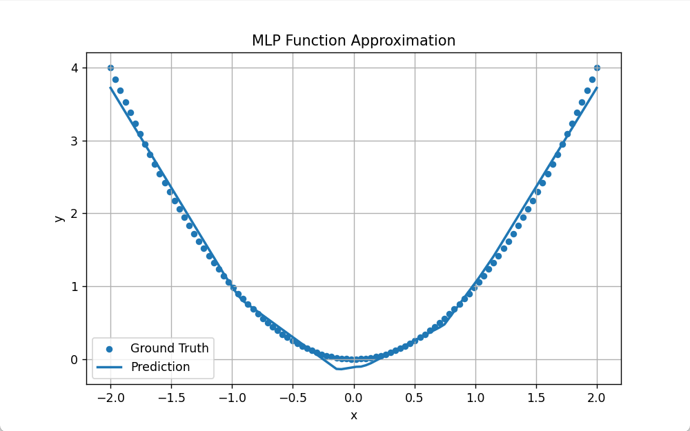
如果我我们把数据改成y=x2 ,那么一层Linear就无法拟合了,直线无法拟合抛物线,要加入ReLU
py
import numpy as np
import matplotlib.pyplot as plt

from layers.Linear import Linear
from losses.MSELoss import MSELoss
from optim.SGD import SGD
from core.Sequential import Sequential
from layers.Relu import RelU

#准备数据
# x
x = np.linspace(
    -2,
    2,
    100
).reshape(-1,1)

y = x ** 2

print(x.shape)
print(y.shape)

#创建模型
model = Sequential(
    Linear(1,16),
    RelU(),
    Linear(16,1)
)


#损失函数
criterion = MSELoss()

#优化器
optimizer = SGD(
    model.parameters(),
    lr=0.001
)

#训练
epochs = 50000
# 记录每一轮的 Loss
loss_history = []

for epoch in range(epochs):
    optimizer.zero_grad()
    pred = model.forward(x)
    loss = criterion.forward(pred,y)
    loss_history.append(loss)
    grad = criterion.backward()
    model.backward(grad)
    optimizer.step()
    if epoch % 1000 == 0:
        print(
            f"Epoch {epoch:4d} "
            f"Loss = {loss:.6f}"
        )


print("\n训练完成!")
for i, p in enumerate(model.parameters()):
    print(f"Parameter {i}:")
    print(p.data)

pred = model.forward(x)
plt.figure(figsize=(8,5))

plt.plot(loss_history)

plt.title("Training Loss")

plt.xlabel("Epoch")

plt.ylabel("MSE Loss")

plt.grid(True)

plt.show()

plt.figure(figsize=(8,5))

plt.scatter(
    x,
    y,
    label="Ground Truth",
    s=20
)

plt.plot(
    x,
    pred,
    linewidth=2,
    label="Prediction"
)

plt.title("MLP Function Approximation")

plt.xlabel("x")

plt.ylabel("y")

plt.legend()

plt.grid(True)

plt.show()Epoch 49000 Loss = 0.006428
训练完成!
Parameter 0:
[[-0.50197322 -0.67009446 -0.74016847 -0.25416111 -0.39211176 0.87908175
-2.38556256 -0.01171286 -1.18215641 -0.43516629 1.54061235 -2.16118324
1.39171419 0.22940398 0.09856138 0.41403664]]
Parameter 1:
[-1.18714420e-02 1.33807927e-03 -3.40873018e-01 -1.31516838e-02
3.06792333e-03 -1.59289906e-02 -9.88716054e-04 -1.50153717e-02
-1.20475265e+00 -9.49103981e-02 -5.96648448e-03 -2.51596044e-01
-1.19184341e+00 -2.44442598e-02 -8.03678294e-02 -2.44177319e-02]
Parameter 2:
[[-0.50350486]
[-0.28671426]
[ 0.44259733]
[-0.49974625]
[-0.01428002]
[-0.00180557]
[ 0.05806183]
[ 0.02477452]
[ 1.37574844]
[ 0.16479115]
[ 0.54326201]
[ 0.6127524 ]
[ 1.59486703]
[-0.24463643]
[-0.78134983]
[-0.21404037]]
Parameter 3:
[-0.05764537]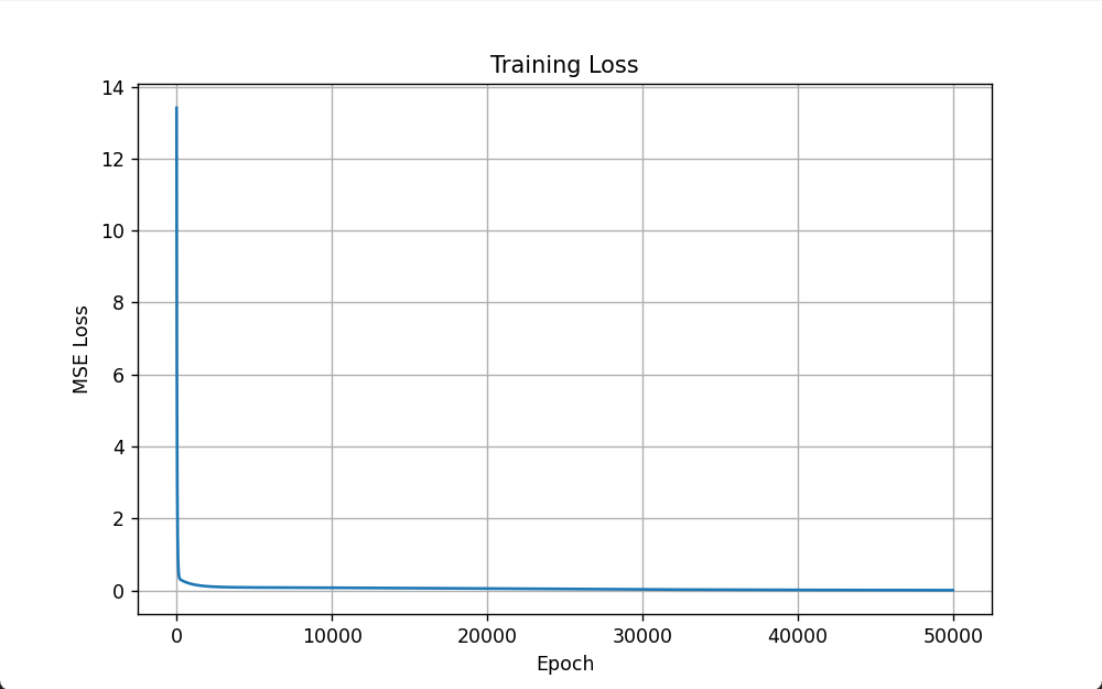
分类任务test;
py
import numpy as np
import matplotlib.pyplot as plt

from core.Sequential import Sequential
from layers.Linear import Linear
from layers.Relu import RelU
from losses.CrossEntropyLoss import CrossEntropyLoss
from optim.SGD import SGD

# 构造数据集
np.random.seed(42)
# 第一类(标签0)
class0 = np.random.randn(100, 2) * 0.5 + np.array([-2, -2])
# 第二类(标签1)
class1 = np.random.randn(100, 2) * 0.5 + np.array([2, 2])
# 合并数据
x = np.vstack((class0, class1))
# 标签
y = np.array([0] * 100 + [1] * 100)

print(x.shape)      # (200,2)
print(y.shape)      # (200,)

# 创建模型
model = Sequential(
    Linear(2, 16),
    RelU(),
    Linear(16, 2)
)

# 损失函数
criterion = CrossEntropyLoss()

# 优化器
optimizer = SGD(
    model.parameters(),
    lr=0.01
)

# 开始训练

epochs = 5000

loss_history = []

for epoch in range(epochs):

    optimizer.zero_grad()

    logits = model.forward(x)

    loss = criterion.forward(logits, y)

    loss_history.append(loss)

    grad = criterion.backward()

    model.backward(grad)

    optimizer.step()

    if epoch % 500 == 0:

        print(f"Epoch {epoch:4d} Loss = {loss:.6f}")

# 预测

logits = model.forward(x)

pred = np.argmax(logits, axis=1)

accuracy = np.mean(pred == y)

print()

print(f"Accuracy: {accuracy * 100:.2f}%")

# Loss 曲线

plt.figure(figsize=(8,5))

plt.plot(loss_history)

plt.title("Training Loss")

plt.xlabel("Epoch")

plt.ylabel("Cross Entropy Loss")

plt.grid(True)

plt.show()

# 分类结果

plt.figure(figsize=(6,6))

plt.scatter(
    x[pred == 0, 0],
    x[pred == 0, 1],
    label="Predict Class 0",
    alpha=0.8
)

plt.scatter(
    x[pred == 1, 0],
    x[pred == 1, 1],
    label="Predict Class 1",
    alpha=0.8
)

plt.legend()

plt.title("Classification Result")

plt.xlabel("x1")

plt.ylabel("x2")

plt.grid(True)

plt.show()

# 绘制决策边界
# 生成二维网格
xx, yy = np.meshgrid(
    np.linspace(-4, 4, 300),
    np.linspace(-4, 4, 300)
)
# 拼成 (90000,2)
grid = np.c_[
    xx.ravel(),
    yy.ravel()
]
# 网络预测
logits = model.forward(grid)
pred = np.argmax(logits, axis=1)
# 恢复成网格
pred = pred.reshape(xx.shape)
# 绘图
plt.figure(figsize=(8,6))
# 背景颜色(决策区域)
plt.contourf(
    xx,
    yy,
    pred,
    alpha=0.3
)
# 第一类
plt.scatter(
    class0[:,0],
    class0[:,1],
    label="Class 0"
)
# 第二类
plt.scatter(
    class1[:,0],
    class1[:,1],
    label="Class 1"
)

plt.title("Decision Boundary")

plt.xlabel("x1")

plt.ylabel("x2")

plt.legend()

plt.grid(True)

plt.show()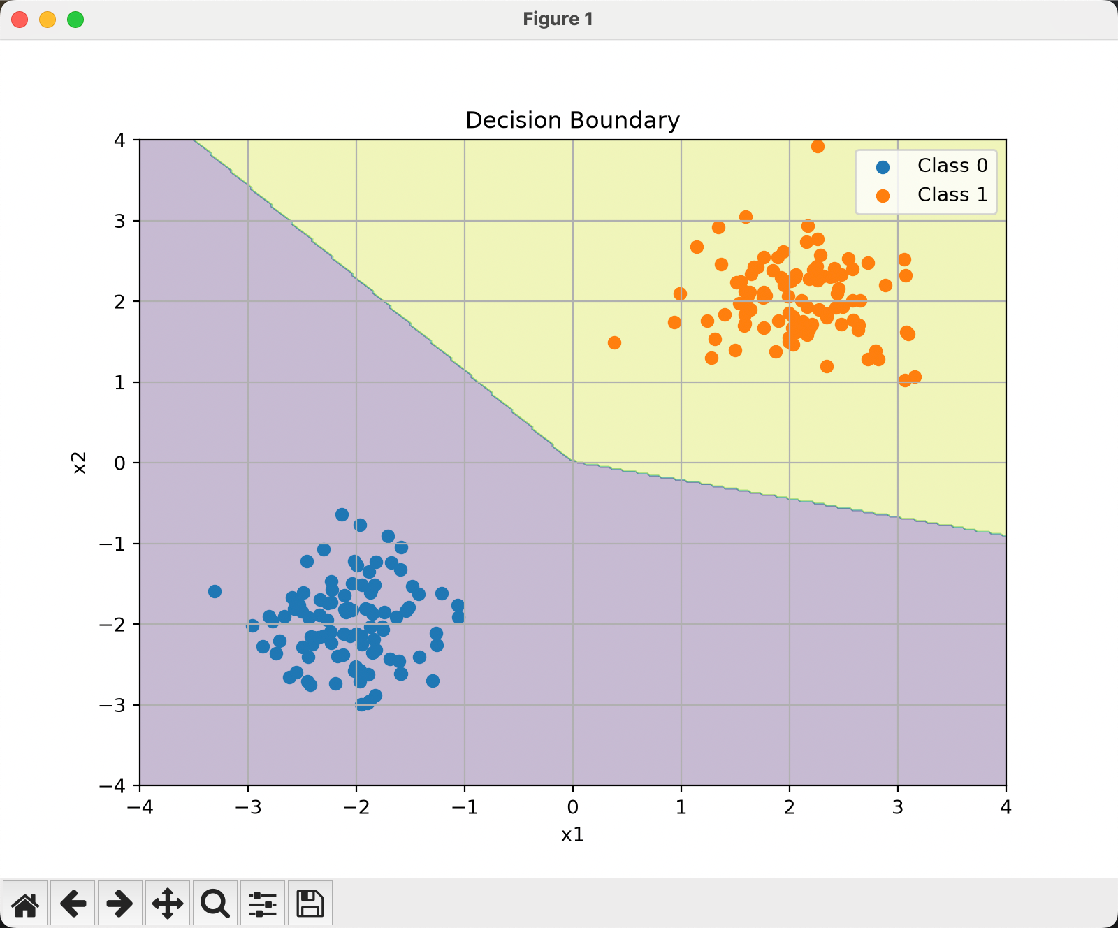
七、batchNorm
BatchNorm 可以加快训练、提高稳定性。
为什么?如何提高的?
先来看一个简单的神经网络。
输入
 │
 ▼
Linear
 │
 ▼
ReLU
 │
 ▼
Linear
 │
 ▼
Loss
假设第一层 Linear 的输出如下:
第一轮训练:
[
100,
120,
130,
150
]
第二轮训练(参数更新后):
[
300,
330,
350,
380
]
第三轮训练:
[
-50,
-20,
10,
40
]
可以发现:
第一层输出的数据分布一直在变化(权重、bias参数更新了)
这意味着:
第二层网络每一次训练,都要重新适应新的输入分布。
训练速度就会变慢,甚至不稳定。
这就是 BatchNorm 想解决的问题。
batchNorm:
把每一个 Batch 的数据标准化,让它的均值接近 0,方差接近 1。
例如:
原始数据:
100
120
130
150
均值:
125减去均值:
-25
-5
5
25
再除以标准差:
-1.2
-0.3
0.2
1.3
于是得到:
均值 = 0

方差 = 1
这就是 Batch Normalization。
BatchNorm 不是对整个数据集做标准化。
也不是对每个样本分别标准化。
而是:
对一个 Batch 中,同一个特征进行标准化。
例如:
一个 Batch:
shape = (4,2)表示:
4 个样本

每个样本有 2 个特征
数据如下:
[
 [100,20],
 [120,30],
 [130,25],
 [150,35]
]
BatchNorm 会分别计算:
第一列:
100
120
130
150
计算:
mean1

var1
第二列:
20
30
25
35
计算:
mean2

var2
所以:
BatchNorm 是按列(特征)标准化。
而不是按行(样本)标准化。
很多人会认为:
BatchNorm 的目的就是把一个 Batch 内的数据统一一下。
其实:这只是实现方式。
真正的目的是:
让后一层神经网络每次都看到相似的数据分布。
例如:
第一层输出:
第一次:
均值 = 125第二次:
均值 = 340第三次:
均值 = -5如果没有 BatchNorm:
第二层每一次都要重新适应新的输入。
如果加入 BatchNorm:
无论第一层输出什么:
100
120
130
150
还是:
300
330
350
380
都会被标准化成:
-1.2
-0.3
0.2
1.3
于是:
第二层每次接收到的数据分布都比较稳定。
训练更快。
BatchNorm 的数学公式
设输入为:X
shape:
(batch_size, features)例如:
(32,128)表示:
32 个样本

128 个特征
第一步:计算均值
对于每个特征:
μ = 1 N ∑ i = 1 N x i \mu=\frac1N\sum_{i=1}^{N}x_i μ=N1i=1∑Nxi
python
mean = np.mean(x, axis=0)为什么是 axis=0?
因为要统计:
每一个特征在整个 Batch 上的均值。
第二步:计算方差
σ 2 = 1 N ∑ i = 1 N ( x i − μ ) 2 \sigma^2=\frac1N\sum_{i=1}^{N}(x_i-\mu)^2 σ2=N1i=1∑N(xi−μ)2
代码:
python
var = np.var(x, axis=0)第三步:标准化
x ^ = x − μ σ 2 + ε \hat{x}=\frac{x-\mu}{\sqrt{\sigma^2+\varepsilon}} x^=σ2+ε x−μ
其中:
ε = 1e-5作用是防止除零。
第四步:恢复表达能力
如果只进行标准化:
所有数据都会变成:
均值 = 0

方差 = 1
神经网络的表达能力反而会下降。
因此:
BatchNorm 又增加了两个可以学习的参数:
γ(gamma)

β(beta)
最终输出:
y = γ x ^ + β y=\gamma\hat{x}+\beta y=γx^+β
-
γ:控制缩放(Scale)。
-
β:控制平移(Shift)。
例如:
标准化后:
[-1,0,1]如果:
γ = 3

β = 5
那么:
3×[-1,0,1]+5

=

[2,5,8]
因此:
BatchNorm 并不会限制网络的表达能力。
BatchNorm 需要学习哪些参数?
只有两个:
γ(gamma)

β(beta)
而:
mean

var
不是模型参数。
训练阶段和测试阶段有什么区别?
训练阶段(train)
每一个 Batch:
都会重新计算:
mean

var
然后进行标准化。
同时:
维护两个全局统计量:
running_mean

running_var
不断更新。
测试阶段(eval)
测试时可能只有:
batch_size = 1甚至:
只有一张图片。
这时候:
不能再计算 Batch 的均值和方差。
因此:
直接使用训练阶段保存的:
running_mean

running_var
进行标准化。
BatchNorm 在代码中的 Forward 流程
输入 X
      │
      ▼
计算 mean
      │
      ▼
计算 var
      │
      ▼
标准化
      │
      ▼
乘 γ
      │
      ▼
加 β
      │
      ▼
输出 Y
python
mean = np.mean(x, axis=0)

var = np.var(x, axis=0)

x_hat = (x - mean) / np.sqrt(var + eps)

out = gamma * x_hat + beta
backward推导,
先看计算图:
            x
            │
      ┌─────┴─────┐
      │           │
      ▼           ▼
    mean        variance
      │           │
      └─────┬─────┘
            ▼
      x - mean
            │
            ▼
     divide sqrt(var)
            │
            ▼
         x_hat
            │
      gamma*x_hat
            │
      + beta
            │
            ▼
           out
已知:
∂ L ∂ o u t \frac{\partial L}{\partial out} ∂out∂L
现在求dβ
y = γ x ^ + β y = \gamma \hat x + \beta y=γx^+β
所以:
∂ y ∂ β = 1 \frac{\partial y}{\partial \beta}=1 ∂β∂y=1
d β = ∑ d o u t d\beta = \sum dout dβ=∑dout
求 γ \gamma γ:
y = γ x ^ + β y = \gamma \hat x + \beta y=γx^+β
所以:
∂ y ∂ γ = x ^ \frac{\partial y}{\partial \gamma}=\hat x ∂γ∂y=x^
d γ = ∑ d o u t × x ^ d\gamma = \sum dout \times \hat x dγ=∑dout×x^
然后求x就复杂了
        x
      / | \
     /  |  \
 mean  var x-mean
x:
既决定均值。又决定方差。还决定自己。
x的backward
          dout
            │
            ▼
      y = γx̂ + β
      │        │
      │        └──── dbeta
      │
      ├──── dgamma
      │
      ▼
      dx_hat
      │
      ▼
x_hat = x_mu * inv
      │         │
      │         ▼
      │      dinv
      │         │
      ▼         ▼
   dx_mu1      dstd
        \        │
         \       ▼
          \    dvar
           \     │
            ▼    ▼
             dx_mu2
                 │
                 ▼
             dx_mu
                 │
                 ▼
              dmean
                 │
                 ▼
                 dx
py
import numpy as np
from core.Module import Module
from core.Parameter import Parameter


class BatchNorm(Module):

    def __init__(self,
                 num_features,
                 eps=1e-5,
                 momentum=0.9):

        self.eps = eps
        self.momentum = momentum

        # 可学习参数
        self.gamma = Parameter(
            np.ones(num_features)
        )

        self.beta = Parameter(
            np.zeros(num_features)
        )

        # 测试使用
        self.running_mean = np.zeros(num_features)
        self.running_var = np.ones(num_features)

        self.training = True

    def forward(self, x):

        if self.training:

            N = x.shape[0]

            # Step1
            # mean

            mean = np.mean(
                x,
                axis=0
            )

            # Step2
            # x - mean

            x_mu = x - mean

            # Step3
            # square

            sq = x_mu ** 2

            # Step4
            # variance

            var = np.mean(
                sq,
                axis=0
            )

            # Step5
            # sqrt

            std = np.sqrt(
                var + self.eps
            )

            # Step6
            # inverse

            inv_std = 1.0 / std

            # Step7
            # normalize

            x_hat = x_mu * inv_std

            # Step8
            # gamma * x_hat

            gamma_x = (
                self.gamma.data
                * x_hat
            )

            # Step9
            # + beta

            out = (
                gamma_x
                + self.beta.data
            )

            # 更新running统计量
            self.running_mean = (
                self.momentum * self.running_mean
                + (1 - self.momentum) * mean
            )

            self.running_var = (
                self.momentum * self.running_var
                + (1 - self.momentum) * var
            )

            # cache
            self.x = x
            self.mean = mean
            self.x_mu = x_mu
            self.sq = sq
            self.var = var
            self.std = std
            self.inv_std = inv_std
            self.x_hat = x_hat
            self.gamma_x = gamma_x

            return out

        else:

            x_hat = (
                x - self.running_mean
            ) / np.sqrt(
                self.running_var + self.eps
            )

            out = (
                self.gamma.data * x_hat
                + self.beta.data
            )

            return out

    def backward(self, dout):

        N = dout.shape[0]

        # Step1
        # out = gamma_x + beta

        self.beta.grad = np.sum(
            dout,
            axis=0
        )

        dgamma_x = dout

        # Step2
        # gamma_x = gamma * x_hat

        self.gamma.grad = np.sum(
            dgamma_x * self.x_hat,
            axis=0
        )

        dx_hat = (
            dgamma_x
            * self.gamma.data
        )

        # Step3
        # x_hat = x_mu * inv_std

        dx_mu1 = (
            dx_hat
            * self.inv_std
        )

        dinv_std = np.sum(
            dx_hat * self.x_mu,
            axis=0
        )

        # Step4
        # inv = 1 / std

        dstd = (
            dinv_std
            * (-1.0)
            / (self.std ** 2)
        )

        # Step5
        # std = sqrt(var+eps)

        dvar = (
            dstd
            * 0.5
            / self.std
        )
        # Step6
        # var = mean(square)
        # var = (1/N) * sum(square)

        dsq = (
                np.ones_like(self.sq)
                * dvar
                / N
        )

        # Step7
        # square = x_mu^2

        dx_mu2 = (
                2.0
                * self.x_mu
                * dsq
        )

        # Step8
        # 两条路径汇合
        # x_mu 同时来自:
        # x_hat = x_mu * inv
        # square = x_mu^2

        dx_mu = (
                dx_mu1
                + dx_mu2
        )

        # Step9
        # x_mu = x - mean

        dx1 = dx_mu

        dmean = -np.sum(
            dx_mu,
            axis=0
        )

        # Step10
        # mean = (1/N) sum(x)

        dx2 = (
                np.ones_like(self.x)
                * dmean
                / N
        )

        # Step11
        # 两条路径再次汇合

        dx = (
                dx1
                + dx2
        )

        return dx

    def parameters(self):

        return [
            self.gamma,
            self.beta
        ]

    def train(self):

        self.training = True

    def eval(self):

        self.training = False
八、Conv卷积层
为什么需要卷积?
先看一张图片。
1 2 3 4 5
6 7 8 9 1
2 3 4 5 6
7 8 9 1 2
3 4 5 6 7
shape=(5,5)
每个数字就是一个像素pixel,255白色 0黑色
如果用 Linear 怎么做?
如果把图片送进全连接层。
首先要:
拉直。
1
2
3
4
5
6
...然后Linear(25,100)
意思是25个输入,100个输出
但是如果这个图像平移1个像素,就全变了,Linear不知道他们还是一个东西
卷积认为一次不用看一整张图,只需要看一个小窗口
这个窗口:Sliding Window(滑动窗口)
卷积核(Kernel):一个小矩阵,属于模型参数,weight
卷积核扫描完的图像叫Feature Map(特征图)
一开始kernel是随机初始化,然后不断更新(比如有的检测直线,有的检测竖线,有的检测眼睛)这都是自己学习更新得到的
真实的彩色图片是RGB三通道
输入是
(C,H,W)再加上batch就是
(N,C,H,W) 例(64,3,32,32)就是一次训练64张图片,每个有三通道,每个通道大小是32*32
卷积核形状:
假设:
py
Conv2D(
    in_channels=3,
    out_channels=16,
    kernel_size=3
)那么权重是(16,3,3,3)
16表示16个卷积核,输出16个特征图,3表示每个卷积核同时覆盖3个颜色通道,3*3表示卷积核空间大小
卷积核输出大小:
o u t = H + 2 P − K S + 1 out=\frac{H+2P-K}{S}+1 out=SH+2P−K+1
H:输入高度
K:kernel大小
P:padding(填充0的边距)
S:stride(步长)
py
import numpy as np

from core.Module import Module
from core.Parameter import Parameter


class Conv2D(Module):
    """
    二维卷积层
    输入:
        (N, Cin, H, W)
    输出:
        (N, Cout, Hout, Wout)
    """

    def __init__(
            self,
            in_channels,
            out_channels,
            kernel_size
    ):

        self.in_channels = in_channels
        self.out_channels = out_channels
        self.kernel_size = kernel_size
        weight = np.random.randn(
            out_channels,
            in_channels,
            kernel_size,
            kernel_size
        ) * np.sqrt(
            2.0 / (
                    in_channels
                    * kernel_size
                    * kernel_size
            )
        )

        bias = np.zeros(
            out_channels
        )

        self.W = Parameter(weight)

        self.b = Parameter(bias)

    def forward(self, x):
        self.x = x
        N, C, H, W = x.shape
        K = self.kernel_size
        H_out = H - K + 1

        W_out = W - K + 1
        out = np.zeros(
            (
                N,
                self.out_channels,
                H_out,
                W_out
            )
        )

        for n in range(N):

            for f in range(self.out_channels):

                for i in range(H_out):

                    for j in range(W_out):
                        window = x[
                            n,
                            :,
                            i:i + K,
                            j:j + K
                        ]

                        out[
                            n,
                            f,
                            i,
                            j
                        ] = (
                                np.sum(
                                    window
                                    *
                                    self.W.data[f]
                                )
                                +
                                self.b.data[f]
                        )
        return out

    def backward(self, grad_output):

        self.W.grad = np.zeros_like(self.W.data)

        self.b.grad = np.zeros_like(self.b.data)

        dx = np.zeros_like(self.x)

        N, _, H_out, W_out = grad_output.shape

        K = self.kernel_size

        for n in range(N):
            for f in range(self.out_channels):
                for i in range(H_out):
                    for j in range(W_out):
                        window = self.x[
                            n,
                            :,
                            i:i + K,
                            j:j + K
                        ]
                        self.b.grad[f] += grad_output[n, f, i, j]
                        self.W.grad[f] += (
                                window
                                * grad_output[n, f, i, j]
                        )
                        dx[
                            n,
                            :,
                            i:i + K,
                            j:j + K
                        ] += (
                                self.W.data[f]
                                * grad_output[n, f, i, j]
                        )
        return dx

    def parameters(self):
        return [self.W, self.b]
九、MaxPool池化层
在一个小窗口里,只取最大值,做"降采样"。
py
import numpy as np
from core.Module import Module


class MaxPool2D(Module):

    def __init__(self, kernel_size=2, stride=2):
        self.kernel_size = kernel_size
        self.stride = stride

        # 用于 backward
        self.x = None
        self.mask = None

    def forward(self, x):
        self.x = x

        N, C, H, W = x.shape
        K = self.kernel_size
        S = self.stride

        H_out = H // S
        W_out = W // S

        out = np.zeros((N, C, H_out, W_out))
        self.mask = np.zeros_like(x)

        for n in range(N):
            for c in range(C):
                for i in range(H_out):
                    for j in range(W_out):

                        h_start = i * S
                        h_end = h_start + K

                        w_start = j * S
                        w_end = w_start + K

                        window = x[n, c, h_start:h_end, w_start:w_end]

                        max_val = np.max(window)
                        out[n, c, i, j] = max_val

                        # 记录 max 位置(反向传播用)
                        mask = (window == max_val)
                        self.mask[n, c, h_start:h_end, w_start:w_end] += mask

        return out

    def backward(self, grad_output):

        dx = np.zeros_like(self.x)

        N, C, H_out, W_out = grad_output.shape
        K = self.kernel_size
        S = self.stride

        for n in range(N):
            for c in range(C):
                for i in range(H_out):
                    for j in range(W_out):

                        h_start = i * S
                        w_start = j * S

                        grad = grad_output[n, c, i, j]

                        dx[n, c,
                           h_start:h_start+K,
                           w_start:w_start+K] += (
                            self.mask[n, c,
                                      h_start:h_start+K,
                                      w_start:w_start+K]
                            * grad
                        )

        return dx

    def parameters(self):
        return []
跑了个MINIST数据集,发现非常慢,原因是没用im2col版本的conv
py
import numpy as np
from core.Module import Module
from core.Parameter import Parameter


class Conv2D(Module):

    def __init__(self, in_channels, out_channels, kernel_size):
        self.in_channels = in_channels
        self.out_channels = out_channels
        self.kernel_size = kernel_size

        K = kernel_size

        weight = np.random.randn(
            out_channels,
            in_channels,
            K,
            K
        ) * np.sqrt(2.0 / (in_channels * K * K))

        bias = np.zeros(out_channels)

        self.W = Parameter(weight)
        self.b = Parameter(bias)

    # =========================
    # im2col
    # =========================
    def im2col(self, x):
        N, C, H, W = x.shape
        K = self.kernel_size

        H_out = H - K + 1
        W_out = W - K + 1

        cols = []

        for n in range(N):
            for i in range(H_out):
                for j in range(W_out):

                    patch = x[
                        n,
                        :,
                        i:i+K,
                        j:j+K
                    ]

                    cols.append(patch.flatten())

        return np.array(cols), H_out, W_out

    # =========================
    # forward
    # =========================
    def forward(self, x):
        self.x = x

        N, C, H, W = x.shape
        K = self.kernel_size

        self.x_col, H_out, W_out = self.im2col(x)

        W_col = self.W.data.reshape(self.out_channels, -1)

        out = self.x_col @ W_col.T + self.b.data

        out = out.reshape(N, H_out, W_out, self.out_channels)
        out = out.transpose(0, 3, 1, 2)

        return out

    # =========================
    # backward
    # =========================
    def backward(self, grad_output):

        N, C, H, W = self.x.shape
        K = self.kernel_size

        H_out = H - K + 1
        W_out = W - K + 1

        grad_output = grad_output.transpose(0, 2, 3, 1)
        grad_output = grad_output.reshape(-1, self.out_channels)

        W_col = self.W.data.reshape(self.out_channels, -1)

        # =========================
        # 1. bias grad
        # =========================
        self.b.grad = np.sum(grad_output, axis=0)

        # =========================
        # 2. weight grad
        # =========================
        self.W.grad = grad_output.T @ self.x_col
        self.W.grad = self.W.grad.reshape(self.W.data.shape)

        # =========================
        # 3. dx
        # =========================
        dx_col = grad_output @ W_col
        dx = np.zeros_like(self.x)

        idx = 0
        for n in range(N):
            for i in range(H_out):
                for j in range(W_out):
                    dx[n, :, i:i+K, j:j+K] += dx_col[idx].reshape(C, K, K)
                    idx += 1

        return dx

    # =========================
    # parameters
    # =========================
    def parameters(self):
        return [self.W, self.b]
替换完了每个batch提速13s左右
py
import numpy as np
from core.summary import summary
from layers.Conv2D import Conv2D
from layers.Relu import RelU
from layers.MaxPool2D import MaxPool2D
from layers.Linear import Linear
from core.Sequential import Sequential
from core.Flatten import Flatten
from losses.MSELoss import MSELoss
from optim.SGD import SGD
import time
from sklearn.datasets import fetch_openml
import matplotlib.pyplot as plt

# =====================
# 数据
# =====================
mnist = fetch_openml("mnist_784", version=1)

X = mnist.data.values.astype(np.float32) / 255.0
y = mnist.target.astype(np.int64)

X = X.reshape(-1, 1, 28, 28)

# one-hot !!!
num_classes = 10
Y = np.zeros((y.shape[0], num_classes))
Y[np.arange(y.shape[0]), y] = 1
X = X[:200]
Y = Y[:200]

# =====================
# 模型
# =====================
model = Sequential(
    Conv2D(1, 8, 3),
    RelU(),
    MaxPool2D(2, 2),

    Conv2D(8, 16, 3),
    RelU(),
    MaxPool2D(2, 2),

    Flatten(),
    Linear(16 * 5 * 5, 128),
    RelU(),
    Linear(128, 10)
)
summary(model, (1, 28, 28))

# =====================
# loss + optimizer
# =====================
criterion = MSELoss()

optimizer = SGD(
    model.parameters(),
    lr=0.01
)


# =====================
# accuracy
# =====================
def accuracy(pred, target):
    pred_label = np.argmax(pred, axis=1)
    true_label = np.argmax(target, axis=1)
    return np.mean(pred_label == true_label)


# =====================
# 训练
# =====================
import time

epochs = 50
batch_size = 64

print("开始训练")
loss_history = []
acc_history = []
for epoch in range(epochs):

    start_time = time.time()

    total_loss = 0
    total_acc = 0
    count = 0

    print(f"\n===== Epoch {epoch} 开始 =====", flush=True)

    for i in range(0, len(X), batch_size):

        batch_idx = i // batch_size

        # if batch_idx % 200 == 0:
        print(f'开始第 {batch_idx} 个 batch训练', flush=True)

        x_batch = X[i:i+batch_size]
        y_batch = Y[i:i+batch_size]

        # forward
        pred = model.forward(x_batch)
        loss = criterion.forward(pred, y_batch)

        # backward
        grad = criterion.backward()
        model.backward(grad)

        optimizer.step()
        optimizer.zero_grad()

        total_loss += loss
        total_acc += accuracy(pred, y_batch)
        count += 1

    end_time = time.time()

    avg_loss = total_loss / count
    avg_acc = total_acc / count
    loss_history.append(avg_loss)
    acc_history.append(avg_acc)
    epoch_time = end_time - start_time

    print(
        f"Epoch {epoch:02d} | "
        f"Loss: {avg_loss:.4f} | "
        f"Acc: {avg_acc:.4f} | "
        f"Time: {epoch_time:.2f}s",
        flush=True
    )

print("训练完成", flush=True)
plt.figure(figsize=(12,5))

# ===== loss =====
plt.subplot(1,2,1)
plt.plot(loss_history)
plt.title("Loss Curve")
plt.xlabel("Epoch")
plt.ylabel("Loss")
plt.grid(True)

# ===== acc =====
plt.subplot(1,2,2)
plt.plot(acc_history)
plt.title("Accuracy Curve")
plt.xlabel("Epoch")
plt.ylabel("Accuracy")
plt.grid(True)

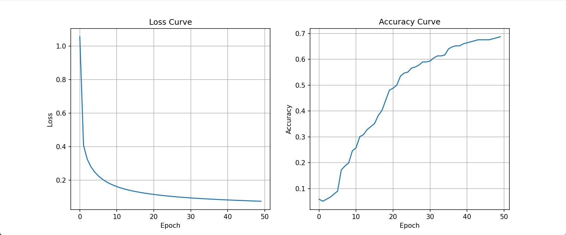
plt.show()===== Epoch 49 开始 =====
开始第 0 个 batch训练
开始第 1 个 batch训练
开始第 2 个 batch训练
开始第 3 个 batch训练
Epoch 49 | Loss: 0.0737 | Acc: 0.6875 | Time: 4.50s
训练完成