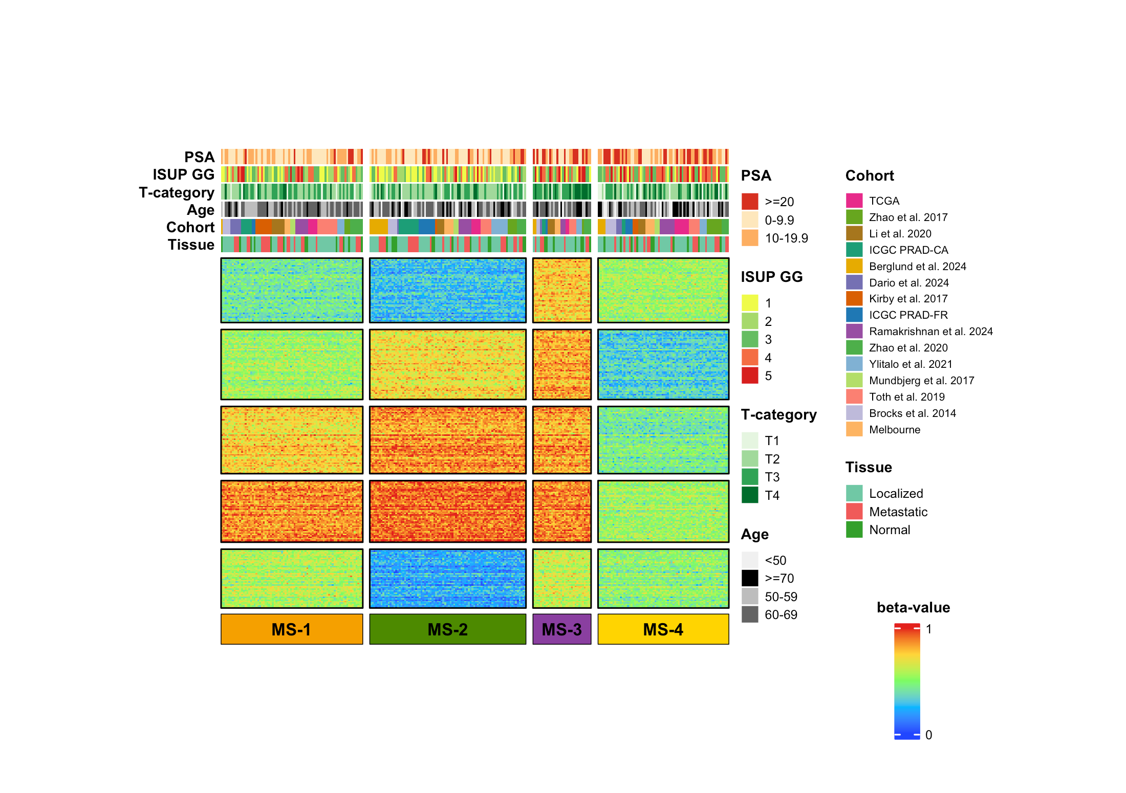
展示多队列样本的分子分型结果:横向是样本,纵向是甲基化特征,顶部叠加临床变量和队列来源,底部标出分型标签。核心是用分块热图把"甲基化模式、临床注释、分型结果"压缩到同一个 panel 里。
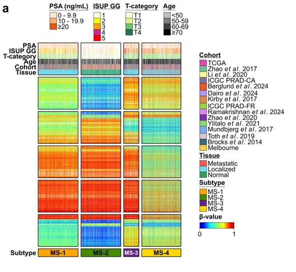
图片来源
| 项目 | 内容 |
|---|---|
| 文章 | The Landscape of Prostate Tumour Methylation |
| 期刊/年份 | bioRxiv / 2025 |
| 图号 | Figure 1a |
| DOI/链接 | https://doi.org/10.1101/2025.02.07.637178 |
这张图展示了前列腺癌样本的甲基化分型结果。图中将样本分成 MS-1、MS-2、MS-3、MS-4 四个亚型,并在顶部加入 PSA、ISUP GG、T-category、Age、Cohort 和 Tissue 等注释信息。
图片解读
这是一张多注释分块热图。
它主要由四部分组成:
- 顶部多行注释条:展示样本临床信息和队列来源。
- 主体热图:展示不同甲基化特征的 beta-value。
- 底部分型条:用颜色标出
MS-1到MS-4。 - 右侧图例区:展示离散注释变量和连续 beta-value 色标。
这类图建议使用 ComplexHeatmap 完成,因为它对顶部注释、列分组、行分块和复杂图例支持更稳定。
输入数据
需要准备三个输入表。
第一个表是甲基化矩阵:input_beta_matrix.csv
| 列名 | 含义 |
|---|---|
feature_id |
CpG 位点、DMR 或甲基化特征编号 |
Sample_001 |
第 1 个样本的 beta-value |
Sample_002 |
第 2 个样本的 beta-value |
... |
其他样本 |
第二个表是样本注释:input_sample_annotation.csv
| 列名 | 含义 |
|---|---|
sample_id |
样本编号,需要与矩阵列名一致 |
subtype |
分型,例如 MS-1、MS-2、MS-3、MS-4 |
psa |
PSA 分组 |
isup_gg |
ISUP 分级 |
t_category |
T 分期 |
age |
年龄分组 |
cohort |
队列来源 |
tissue |
组织类型 |
第三个表是特征注释:input_feature_annotation.csv
| 列名 | 含义 |
|---|---|
feature_id |
特征编号,需要与矩阵行名一致 |
module |
热图行分块,例如 Block-1、Block-2 |
r
library(tidyverse)

sample_anno <- read_csv("input_sample_annotation.csv", show_col_types = FALSE)
feature_anno <- read_csv("input_feature_annotation.csv", show_col_types = FALSE)
beta_df <- read_csv("input_beta_matrix.csv", show_col_types = FALSE)
需要示例数据的后台 添加小编 领取,调整好数据结构,以下代码可以直接复制粘贴运行。
第一步:整理矩阵和分组顺序
先固定 MS-1 到 MS-4 的样本顺序,再把 beta-value 表转成矩阵。
r
library(tidyverse)
suppressPackageStartupMessages(library(ComplexHeatmap))
suppressPackageStartupMessages(library(circlize))
library(grid)

sample_anno <- read_csv("input_sample_annotation.csv", show_col_types = FALSE)
feature_anno <- read_csv("input_feature_annotation.csv", show_col_types = FALSE)
beta_df <- read_csv("input_beta_matrix.csv", show_col_types = FALSE)

subtype_levels <- c("MS-1", "MS-2", "MS-3", "MS-4")

sample_anno <- sample_anno |>
  mutate(subtype = factor(subtype, subtype_levels)) |>
  arrange(subtype, cohort, tissue)

mat <- beta_df |>
  column_to_rownames("feature_id") |>
  as.matrix()

mat <- mat[feature_anno$feature_id, sample_anno$sample_id]

row_split <- factor(feature_anno$module, levels = unique(feature_anno$module))
col_split <- sample_anno$subtype
第二步:设置颜色
离散变量使用命名颜色向量,连续 beta-value 使用 colorRamp2()。
r
psa_cols <- c("0-9.9" = "#fee7bc", "10-19.9" = "#fdae61", ">=20" = "#d7301f")
isup_cols <- c("1" = "#efff49", "2" = "#a6d96a", "3" = "#66bd63", "4" = "#f46d43", "5" = "#d7191c")
t_cols <- c("T1" = "#e5f5e0", "T2" = "#a1d99b", "T3" = "#31a354", "T4" = "#006d2c")
age_cols <- c("<50" = "#f0f0f0", "50-59" = "#bdbdbd", "60-69" = "#636363", ">=70" = "#000000")
tissue_cols <- c("Metastatic" = "#f05a59", "Localized" = "#70c8a5", "Normal" = "#33a02c")
subtype_cols <- c("MS-1" = "#f5a000", "MS-2" = "#4c8a00", "MS-3" = "#8a3fa0", "MS-4" = "#ffd400")

cohort_levels <- c(
  "TCGA", "Zhao et al. 2017", "Li et al. 2020", "ICGC PRAD-CA",
  "Berglund et al. 2024", "Dario et al. 2024", "Kirby et al. 2017",
  "ICGC PRAD-FR", "Ramakrishnan et al. 2024", "Zhao et al. 2020",
  "Ylitalo et al. 2021", "Mundbjerg et al. 2017", "Toth et al. 2019",
  "Brocks et al. 2014", "Melbourne"
)

cohort_cols <- setNames(
  c("#e7298a", "#66a61e", "#a6761d", "#1b9e77", "#e6ab02",
    "#7570b3", "#d95f02", "#1f78b4", "#984ea3", "#4daf4a",
    "#80b1d3", "#b3de69", "#fb8072", "#bebada", "#fdb462"),
  cohort_levels
)

beta_col_fun <- colorRamp2(
  c(0, 0.25, 0.5, 0.75, 1),
  c("#2146ff", "#00b7ff", "#7cff62", "#ffd53a", "#e31a1c")
)
第三步:构建顶部注释和底部分型条
顶部注释用 HeatmapAnnotation(),底部的分型色块用 anno_block()。
r
top_anno <- HeatmapAnnotation(
  PSA = sample_anno$psa,
  `ISUP GG` = as.character(sample_anno$isup_gg),
  `T-category` = sample_anno$t_category,
  Age = sample_anno$age,
  Cohort = factor(sample_anno$cohort, cohort_levels),
  Tissue = sample_anno$tissue,
  col = list(
    PSA = psa_cols,
    `ISUP GG` = isup_cols,
    `T-category` = t_cols,
    Age = age_cols,
    Cohort = cohort_cols,
    Tissue = tissue_cols
  ),
  annotation_name_side = "left",
  annotation_name_gp = gpar(fontsize = 7, fontface = "bold"),
  simple_anno_size = unit(2.6, "mm"),
  gap = unit(0.3, "mm"),
  show_legend = TRUE
)

bottom_anno <- HeatmapAnnotation(
  Subtype = anno_block(
    gp = gpar(fill = subtype_cols[subtype_levels], col = "black", lwd = 0.5),
    labels = subtype_levels,
    labels_gp = gpar(fontsize = 8, fontface = "bold", col = "black")
  ),
  annotation_name_side = "left",
  height = unit(5, "mm")
)
第四步:绘制热图主体
这里把 show_heatmap_legend = FALSE 关掉,是为了后面把 beta-value 图例手动放到右下角。
r
ht <- Heatmap(
  mat,
  name = "beta-value",
  col = beta_col_fun,
  top_annotation = top_anno,
  bottom_annotation = bottom_anno,
  row_split = row_split,
  column_split = col_split,
  cluster_rows = FALSE,
  cluster_columns = FALSE,
  cluster_row_slices = FALSE,
  cluster_column_slices = FALSE,
  show_row_names = FALSE,
  show_column_names = FALSE,
  show_heatmap_legend = FALSE,
  row_title = NULL,
  column_title = NULL,
  row_gap = unit(1.15, "mm"),
  column_gap = unit(1.15, "mm"),
  border = TRUE,
  rect_gp = gpar(col = NA),
  heatmap_width = unit(84, "mm"),
  heatmap_height = unit(82, "mm")
)
第五步:手动放置 beta-value 图例
ComplexHeatmap 默认会把热图图例和注释图例放在一起。为了避免挤在 PSA 旁边,可以单独构建一个 Legend(),再用 draw() 放到右下角。
r
beta_lgd <- Legend(
  title = "beta-value",
  col_fun = beta_col_fun,
  at = c(0, 1),
  labels = c("0", "1"),
  direction = "vertical",
  legend_height = unit(19, "mm"),
  legend_width = unit(4, "mm"),
  title_position = "topcenter",
  title_gp = gpar(fontsize = 7, fontface = "bold"),
  labels_gp = gpar(fontsize = 6)
)

draw_main <- function() {
  draw(
    ht,
    heatmap_legend_side = "right",
    annotation_legend_side = "right",
    merge_legends = FALSE,
    padding = unit(c(4, 4, 4, 4), "mm")
  )

  draw(
    beta_lgd,
    x = unit(0.795, "npc"),
    y = unit(0.155, "npc"),
    just = c("left", "center")
  )
}
第六步:导出图片
r
png("result/methylation_subtype_heatmap.png", width = 2200, height = 1550, res = 300, bg = "white")
draw_main()
dev.off()

pdf("result/methylation_subtype_heatmap.pdf", width = 7.35, height = 5.15, bg = "white")
draw_main()
dev.off()
完整代码
r
library(tidyverse)
suppressPackageStartupMessages(library(ComplexHeatmap))
suppressPackageStartupMessages(library(circlize))
library(grid)

dir.create("result", showWarnings = FALSE)

sample_anno <- read_csv("input_sample_annotation.csv", show_col_types = FALSE)
feature_anno <- read_csv("input_feature_annotation.csv", show_col_types = FALSE)
beta_df <- read_csv("input_beta_matrix.csv", show_col_types = FALSE)

ht_opt(
  legend_title_gp = gpar(fontsize = 7, fontface = "bold"),
  legend_labels_gp = gpar(fontsize = 6),
  TITLE_PADDING = unit(c(1, 1), "mm")
)

subtype_levels <- c("MS-1", "MS-2", "MS-3", "MS-4")

sample_anno <- sample_anno |>
  mutate(subtype = factor(subtype, subtype_levels)) |>
  arrange(subtype, cohort, tissue)

mat <- beta_df |>
  column_to_rownames("feature_id") |>
  as.matrix()

mat <- mat[feature_anno$feature_id, sample_anno$sample_id]

row_split <- factor(feature_anno$module, levels = unique(feature_anno$module))
col_split <- sample_anno$subtype

psa_cols <- c("0-9.9" = "#fee7bc", "10-19.9" = "#fdae61", ">=20" = "#d7301f")
isup_cols <- c("1" = "#efff49", "2" = "#a6d96a", "3" = "#66bd63", "4" = "#f46d43", "5" = "#d7191c")
t_cols <- c("T1" = "#e5f5e0", "T2" = "#a1d99b", "T3" = "#31a354", "T4" = "#006d2c")
age_cols <- c("<50" = "#f0f0f0", "50-59" = "#bdbdbd", "60-69" = "#636363", ">=70" = "#000000")
tissue_cols <- c("Metastatic" = "#f05a59", "Localized" = "#70c8a5", "Normal" = "#33a02c")
subtype_cols <- c("MS-1" = "#f5a000", "MS-2" = "#4c8a00", "MS-3" = "#8a3fa0", "MS-4" = "#ffd400")

cohort_levels <- c(
  "TCGA", "Zhao et al. 2017", "Li et al. 2020", "ICGC PRAD-CA",
  "Berglund et al. 2024", "Dario et al. 2024", "Kirby et al. 2017",
  "ICGC PRAD-FR", "Ramakrishnan et al. 2024", "Zhao et al. 2020",
  "Ylitalo et al. 2021", "Mundbjerg et al. 2017", "Toth et al. 2019",
  "Brocks et al. 2014", "Melbourne"
)

cohort_cols <- setNames(
  c("#e7298a", "#66a61e", "#a6761d", "#1b9e77", "#e6ab02",
    "#7570b3", "#d95f02", "#1f78b4", "#984ea3", "#4daf4a",
    "#80b1d3", "#b3de69", "#fb8072", "#bebada", "#fdb462"),
  cohort_levels
)

beta_col_fun <- colorRamp2(
  c(0, 0.25, 0.5, 0.75, 1),
  c("#2146ff", "#00b7ff", "#7cff62", "#ffd53a", "#e31a1c")
)

anno_lgd <- list(
  PSA = list(title_gp = gpar(fontsize = 7, fontface = "bold"), labels_gp = gpar(fontsize = 6),
             grid_width = unit(3, "mm"), grid_height = unit(3, "mm")),
  `ISUP GG` = list(title_gp = gpar(fontsize = 7, fontface = "bold"), labels_gp = gpar(fontsize = 6),
                   grid_width = unit(3, "mm"), grid_height = unit(3, "mm")),
  `T-category` = list(title_gp = gpar(fontsize = 7, fontface = "bold"), labels_gp = gpar(fontsize = 6),
                      grid_width = unit(3, "mm"), grid_height = unit(3, "mm")),
  Age = list(title_gp = gpar(fontsize = 7, fontface = "bold"), labels_gp = gpar(fontsize = 6),
             grid_width = unit(3, "mm"), grid_height = unit(3, "mm")),
  Cohort = list(title_gp = gpar(fontsize = 7, fontface = "bold"), labels_gp = gpar(fontsize = 5.1),
                grid_width = unit(3, "mm"), grid_height = unit(2.7, "mm")),
  Tissue = list(title_gp = gpar(fontsize = 7, fontface = "bold"), labels_gp = gpar(fontsize = 6),
                grid_width = unit(3, "mm"), grid_height = unit(3, "mm"))
)

top_anno <- HeatmapAnnotation(
  PSA = sample_anno$psa,
  `ISUP GG` = as.character(sample_anno$isup_gg),
  `T-category` = sample_anno$t_category,
  Age = sample_anno$age,
  Cohort = factor(sample_anno$cohort, cohort_levels),
  Tissue = sample_anno$tissue,
  col = list(
    PSA = psa_cols,
    `ISUP GG` = isup_cols,
    `T-category` = t_cols,
    Age = age_cols,
    Cohort = cohort_cols,
    Tissue = tissue_cols
  ),
  annotation_name_side = "left",
  annotation_name_gp = gpar(fontsize = 7, fontface = "bold"),
  simple_anno_size = unit(2.6, "mm"),
  gap = unit(0.3, "mm"),
  show_legend = TRUE,
  annotation_legend_param = anno_lgd
)

bottom_anno <- HeatmapAnnotation(
  Subtype = anno_block(
    gp = gpar(fill = subtype_cols[subtype_levels], col = "black", lwd = 0.5),
    labels = subtype_levels,
    labels_gp = gpar(fontsize = 8, fontface = "bold", col = "black")
  ),
  annotation_name_side = "left",
  annotation_name_gp = gpar(fontsize = 7, fontface = "bold"),
  height = unit(5, "mm")
)

ht <- Heatmap(
  mat,
  name = "beta-value",
  col = beta_col_fun,
  top_annotation = top_anno,
  bottom_annotation = bottom_anno,
  row_split = row_split,
  column_split = col_split,
  cluster_rows = FALSE,
  cluster_columns = FALSE,
  cluster_row_slices = FALSE,
  cluster_column_slices = FALSE,
  show_row_names = FALSE,
  show_column_names = FALSE,
  show_heatmap_legend = FALSE,
  row_title = NULL,
  column_title = NULL,
  row_gap = unit(1.15, "mm"),
  column_gap = unit(1.15, "mm"),
  border = TRUE,
  rect_gp = gpar(col = NA),
  heatmap_width = unit(84, "mm"),
  heatmap_height = unit(82, "mm")
)

beta_lgd <- Legend(
  title = "beta-value",
  col_fun = beta_col_fun,
  at = c(0, 1),
  labels = c("0", "1"),
  direction = "vertical",
  legend_height = unit(19, "mm"),
  legend_width = unit(4, "mm"),
  title_position = "topcenter",
  title_gp = gpar(fontsize = 7, fontface = "bold"),
  labels_gp = gpar(fontsize = 6)
)

draw_main <- function() {
  draw(
    ht,
    heatmap_legend_side = "right",
    annotation_legend_side = "right",
    merge_legends = FALSE,
    padding = unit(c(4, 4, 4, 4), "mm")
  )

  draw(
    beta_lgd,
    x = unit(0.795, "npc"),
    y = unit(0.155, "npc"),
    just = c("left", "center")
  )
}

png("result/methylation_subtype_heatmap.png", width = 2200, height = 1550, res = 300, bg = "white")
draw_main()
dev.off()

pdf("result/methylation_subtype_heatmap.pdf", width = 7.35, height = 5.15, bg = "white")
draw_main()
dev.off()
复现结果