书接上回:从本地 Demo 到生产级检索:Milvus 学习笔记(2)
目录
- 搜索
-
- [文本高亮(Text Highlighter)](#文本高亮(Text Highlighter))
- [短语匹配(Phrase Match)](#短语匹配(Phrase Match))
-
- [Milvus Text Match、Phrase Match 与 Full Text Search 区别](#Milvus Text Match、Phrase Match 与 Full Text Search 区别)
- [使用 Embedding List 进行搜索(Search with Embedding Lists)](#使用 Embedding List 进行搜索(Search with Embedding Lists))
-
- [ColBERT 文本检索系统](#ColBERT 文本检索系统)
-
- [Step 1:安装依赖](#Step 1:安装依赖)
- [Step 2:加载 Cohere 数据集](#Step 2:加载 Cohere 数据集)
- [Step 3:按照标题聚合段落](#Step 3:按照标题聚合段落)
- [Step 4:为 Cohere 数据集创建 Collection](#Step 4:为 Cohere 数据集创建 Collection)
- [Step 5:插入 Cohere 数据集](#Step 5:插入 Cohere 数据集)
- [Step 6:搜索 Cohere 数据集](#Step 6:搜索 Cohere 数据集)
- [ColPali 文本检索系统](#ColPali 文本检索系统)
-
- [Step 1:安装依赖](#Step 1:安装依赖)
- [Step 2:加载 Vidore 数据集](#Step 2:加载 Vidore 数据集)
- [Step 3:为页面图片生成 Embedding](#Step 3:为页面图片生成 Embedding)
- [Step 4:为金融报告数据集创建 Collection](#Step 4:为金融报告数据集创建 Collection)
- [Step 5:将金融报告插入 Collection](#Step 5:将金融报告插入 Collection)
- [Step 6:在金融报告中进行搜索](#Step 6:在金融报告中进行搜索)
- 和普通向量搜索的区别
- [Search Iterator(搜索迭代器)](#Search Iterator(搜索迭代器))
- [使用 Partition Key](#使用 Partition Key)
-
- [Milvus Partition Key 机制理解](#Milvus Partition Key 机制理解)
- 总结
搜索
文本高亮(Text Highlighter)
示例(Examples)
在使用 Highlighter 之前,请确保 Collection 已正确配置。
下面示例会创建一个同时支持:
- BM25 全文检索;
- TEXT_MATCH 查询;
的 Collection,并插入示例文档。
c
from pymilvus import (
    MilvusClient,
    DataType,
    Function,
    FunctionType,
    LexicalHighlighter,
)

client = MilvusClient(uri="http://localhost:19530")
COLLECTION_NAME = "highlighter_demo"

# Clean up existing collection
if client.has_collection(COLLECTION_NAME):
    client.drop_collection(COLLECTION_NAME)

# Define schema
schema = client.create_schema(enable_dynamic_field=False)
schema.add_field(field_name="id", datatype=DataType.INT64, is_primary=True, auto_id=True)
schema.add_field(
    field_name="text",
    datatype=DataType.VARCHAR,
    max_length=2000,
    enable_analyzer=True,  # Required for BM25
    enable_match=True,     # Required for TEXT_MATCH
)
schema.add_field(field_name="sparse_vector", datatype=DataType.SPARSE_FLOAT_VECTOR)

# Add BM25 function
schema.add_function(Function(
    name="text_bm25",
    function_type=FunctionType.BM25,
    input_field_names=["text"],
    output_field_names=["sparse_vector"],
))

# Create index
index_params = client.prepare_index_params()
index_params.add_index(
    field_name="sparse_vector",
    index_type="SPARSE_INVERTED_INDEX",
    metric_type="BM25",
    params={"inverted_index_algo": "DAAT_MAXSCORE", "bm25_k1": 1.2, "bm25_b": 0.75},
)

client.create_collection(collection_name=COLLECTION_NAME, schema=schema, index_params=index_params)

# Insert sample documents
docs = [
    "my first test doc",
    "my second test doc",
    "my first test doc. Milvus is an open-source vector database built for GenAI applications.",
    "my second test doc. Milvus is an open-source vector database that suits AI applications "
    "of every size from running a demo chatbot to building web-scale search.",
]
client.insert(collection_name=COLLECTION_NAME, data=[{"text": t} for t in docs])
print(f"✓ Collection created with {len(docs)} documents\n")

# Helper for search params
SEARCH_PARAMS = {"metric_type": "BM25", "params": {"drop_ratio_search": 0.0}}

# Expected output:
# ✓ Collection created with 4 documents
示例 1:高亮 BM25 全文检索中的搜索词
该示例展示如何在 BM25 全文检索中高亮搜索词。
说明:
- BM25 全文检索使用
"test"作为搜索词; - Highlighter 会将所有匹配到的
"test"使用{}包裹。
python
highlighter = LexicalHighlighter(
    pre_tags=["{"],
    post_tags=["}"],
    highlight_search_text=True,  # 高亮 BM25 查询词
)

results = client.search(
    collection_name=COLLECTION_NAME,
    data=["test"],
    anns_field="sparse_vector",
    limit=10,
    search_params=SEARCH_PARAMS,
    output_fields=["text"],
    highlighter=highlighter,
)

for hit in results[0]:
    print(f"  {hit.get('highlight', {}).get('text', [])}")
print()
示例 2:高亮过滤查询中的词
该示例展示如何高亮 TEXT_MATCH 过滤条件匹配的词。
说明:
-
BM25 全文检索使用
"test"作为查询词; -
highlight_query参数额外添加"my doc"到高亮列表; -
Highlighter 会将所有匹配词:
mytestdoc
使用
{}包裹。
python
highlighter = LexicalHighlighter(
    pre_tags=["{"],
    post_tags=["}"],
    highlight_search_text=True,   # 同时高亮 BM25 查询词
    highlight_query=[             # 额外需要高亮的 TEXT_MATCH 词
        {"type": "TextMatch", "field": "text", "text": "my doc"},
    ],
)

results = client.search(
    collection_name=COLLECTION_NAME,
    data=["test"],
    anns_field="sparse_vector",
    limit=10,
    search_params=SEARCH_PARAMS,
    output_fields=["text"],
    highlighter=highlighter,
)

for hit in results[0]:
    print(f"  {hit.get('highlight', {}).get('text', [])}")
print()
示例 3:以片段形式返回高亮结果
该示例中,查询词为:
text
Milvus并通过以下配置返回高亮片段:
-
fragment_offset- 在第一个高亮位置前保留最多 20 个字符作为上下文。
- 默认值为
0。
-
fragment_size- 限制每个片段长度约为 60 个字符。
- 默认值为
100。
-
num_of_fragments- 限制每个文本值返回的片段数量。
- 默认值为
5。
python
highlighter = LexicalHighlighter(
    pre_tags=["{"],
    post_tags=["}"],
    highlight_search_text=True,
    fragment_offset=20,  # 匹配词前保留 20 个字符
    fragment_size=60,    # 每个片段最大约 60 个字符
)

results = client.search(
    collection_name=COLLECTION_NAME,
    data=["Milvus"],
    anns_field="sparse_vector",
    limit=10,
    search_params=SEARCH_PARAMS,
    output_fields=["text"],
    highlighter=highlighter,
)

for i, hit in enumerate(results[0]):
    frags = hit.get('highlight', {}).get('text', [])
    print(f"  Doc {i+1}: {frags}")
print()
示例 4:多查询高亮(Multi-query Highlighting)
当 BM25 全文检索使用多个查询词时,每个查询的结果会独立进行高亮。
规则:
- 第一个查询结果只高亮自己的搜索词;
- 第二个查询结果只高亮自己的搜索词;
- 依此类推。
所有查询共享同一个 Highlighter 配置,但会分别应用。
示例:
- 第一个查询高亮
"test"; - 第二个查询高亮
"Milvus"。
python
highlighter = LexicalHighlighter(
    pre_tags=["{"],
    post_tags=["}"],
    highlight_search_text=True,
)

results = client.search(
    collection_name=COLLECTION_NAME,
    data=["test", "Milvus"],  # 两个查询
    anns_field="sparse_vector",
    limit=2,
    search_params=SEARCH_PARAMS,
    output_fields=["text"],
    highlighter=highlighter,
)

for nq_idx, hits in enumerate(results):
    query_term = ["test", "Milvus"][nq_idx]
    print(f"  Query '{query_term}':")
    for hit in hits:
        print(f"    {hit.get('highlight', {}).get('text', [])}")
print()
示例 5:自定义 HTML 标签
Highlighter 支持任意标签,例如适用于 Web UI 的 HTML 标签。
这在浏览器中渲染搜索结果时非常有用。
python
highlighter = LexicalHighlighter(
    pre_tags=["<mark>"],
    post_tags=["</mark>"],
    highlight_search_text=True,
)

results = client.search(
    collection_name=COLLECTION_NAME,
    data=["test"],
    anns_field="sparse_vector",
    limit=2,
    search_params=SEARCH_PARAMS,
    output_fields=["text"],
    highlighter=highlighter,
)

for hit in results[0]:
    print(f"  {hit.get('highlight', {}).get('text', [])}")
print()
预期输出:
text
[
    '<mark>test</mark> doc'
]

[
    '<mark>test</mark> doc'
]
短语匹配(Phrase Match)
短语匹配允许你搜索包含查询词组的文档。默认情况下,词语必须按照相同的顺序出现,并且彼此直接相邻。例如,查询短语 "robotics machine learning" 可以匹配类似 "...typical robotics machine learning models..." 的文本,其中 "robotics"、"machine" 和 "learning" 按顺序连续出现,中间没有其他词。
然而,在实际场景中,严格的短语匹配可能过于限制。例如,你可能希望匹配类似 "...machine learning models widely adopted in robotics..." 的文本。这里虽然包含相同的关键词,但它们并不是连续出现,也不是原始顺序。为了解决这个问题,Phrase Match 支持 slop 参数,用于提供更灵活的匹配方式。slop 值表示短语中词语之间允许存在的位置偏移数量。例如,当 slop=1 时,查询 "machine learning" 可以匹配类似 "...machine deep learning..." 的文本,其中一个词("deep")位于原始两个词之间。
Phrase Match 基于 Tantivy 搜索引擎库实现,通过分析文档中词语的位置信息完成匹配。其流程如下:
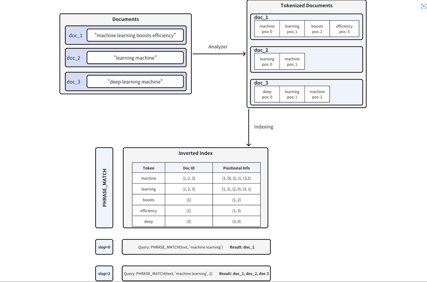
-
文档分词(Document Tokenization)
当向 Milvus 插入文档时,Analyzer 会将文本拆分为 Token(单词或词项),并记录每个 Token 的位置信息。
例如,
doc_1会被分词为:text["machine" (pos=0), "learning" (pos=1), "boosts" (pos=2), "efficiency" (pos=3)] -
创建倒排索引(Inverted Index Creation)
Milvus 会创建倒排索引,将每个 Token 映射到包含该 Token 的文档,以及该 Token 在文档中的位置。
-
短语匹配(Phrase Matching)
执行短语查询时,Milvus 会通过倒排索引查找每个 Token,并检查它们的位置,以判断它们是否按照正确顺序和距离出现。
slop参数控制匹配 Token 之间允许的最大位置偏移:-
slop = 0表示 Token 必须按照准确顺序出现,并且必须直接相邻(即中间不能有额外词语)。例如,只有
doc_1(machine位于 pos=0,learning位于 pos=1)能够精确匹配。 -
slop = 2表示匹配 Token 之间允许最多两个位置的偏移或顺序调整。这允许:
- 反向顺序(例如 "learning machine");
- Token 之间存在较小间隔。
因此,
doc_1、doc_2(learning位于 pos=0,machine位于 pos=1)以及doc_3(learning位于 pos=1,machine位于 pos=2)都会匹配。
-
Phrase Match 使用 VARCHAR 字段类型,即 Milvus 中的字符串数据类型。要启用短语匹配,需要像 Text Match 一样,在 Collection Schema 中将 enable_analyzer 和 enable_match 参数都设置为 True。
要为指定的 VARCHAR 字段启用 Phrase Match,需要在定义字段 Schema 时,将 enable_analyzer 和 enable_match 参数都设置为 True。该配置会让 Milvus 对文本进行分词,并创建包含位置信息的倒排索引,以支持高效的短语匹配。
下面是启用 Phrase Match 的 Schema 定义示例:
python
from pymilvus import MilvusClient, DataType

# 创建新的 Collection Schema
schema = MilvusClient.create_schema(enable_dynamic_field=False)

schema.add_field(
    field_name="id",
    datatype=DataType.INT64,
    is_primary=True,
    auto_id=True
)

# 添加配置用于短语匹配的 VARCHAR 字段
schema.add_field(
    field_name='text',                 # 字段名称
    datatype=DataType.VARCHAR,         # 字段类型设置为 VARCHAR(字符串)
    max_length=1000,                   # 字符串最大长度
    enable_analyzer=True,              # 开启文本分析(分词)
    enable_match=True                  # 开启用于短语匹配的倒排索引
)

schema.add_field(
    field_name="embeddings",
    datatype=DataType.FLOAT_VECTOR,
    dim=5
)
可选:配置 Analyzer
Phrase Match 的准确性很大程度上取决于用于文本分词的 Analyzer。不同 Analyzer 适用于不同语言和文本格式,会影响 Token 的切分方式以及位置准确性。为具体使用场景选择合适的 Analyzer,可以优化 Phrase Match 的效果。
默认情况下,Milvus 使用 standard analyzer,该 Analyzer 会根据空格和标点符号对文本进行分词,删除长度超过 40 个字符的 Token,并将文本转换为小写。默认使用时无需额外参数。详情参考 Standard Analyzer。
如果应用需要指定 Analyzer,可以通过 analyzer_params 参数进行配置。例如,下面展示了如何为英文文本的 Phrase Match 配置 English Analyzer:
python
# 定义英文分词 Analyzer 参数
analyzer_params = {
    "type": "english"
}

# 添加启用 English Analyzer 的 VARCHAR 字段
schema.add_field(
    field_name='text',                 # 字段名称
    datatype=DataType.VARCHAR,         # 字段类型设置为 VARCHAR
    max_length=1000,                   # 字符串最大长度
    enable_analyzer=True,              # 开启文本分析
    analyzer_params=analyzer_params,   # 指定 Analyzer 配置
    enable_match=True                  # 开启用于短语匹配的倒排索引
)
Milvus 支持多种针对不同语言和使用场景优化的 Analyzer。
当已经在 Collection Schema 中为 VARCHAR 字段启用了 match 后,可以使用 PHRASE_MATCH 表达式执行短语匹配。
PHRASE_MATCH 表达式不区分大小写,可以使用:
text
PHRASE_MATCH或者:
text
phrase_match使用 PHRASE_MATCH 表达式时,需要指定搜索字段、短语以及可选的灵活度参数(slop)。
语法:
text
PHRASE_MATCH(field_name, phrase, slop)参数说明:
-
field_name:执行短语匹配的VARCHAR字段名称。 -
phrase:需要搜索的精确短语。 -
slop(可选):整数,表示匹配 Token 时允许的最大位置偏移数量。-
0(默认):仅匹配完全一致的短语。例如,过滤条件搜索:
textmachine learning会匹配:
textmachine learning但不会匹配:
textmachine boosts learning或:
textlearning machine -
1:允许较小变化,例如增加一个额外词或轻微的位置偏移。例如,搜索:
textmachine learning会匹配:
textmachine boosts learning(
machine和learning之间存在一个 Token)但不会匹配:
textlearning machine(词语顺序反转)
-
2:允许更大的灵活性,包括词语顺序反转或中间最多存在两个 Token。例如,搜索:
textmachine learning会匹配:
textlearning machine(词语顺序反转)
或:
textmachine quickly boosts learning(
machine和learning之间存在两个 Token)
-
假设有一个名为 tech_articles 的 Collection,其中包含以下五个实体:
| doc_id | text |
|---|---|
| 1 | "Machine learning boosts efficiency in large-scale data analysis" |
| 2 | "Learning a machine-based approach is vital for modern AI progress" |
| 3 | "Deep learning machine architectures optimize computational loads" |
| 4 | "Machine swiftly improves model performance for ongoing learning" |
| 5 | "Learning advanced machine algorithms expands AI capabilities" |
在使用 query() 方法时,PHRASE_MATCH 作为标量过滤条件使用。只有包含指定短语(根据允许的 slop 判断)的文档才会被返回。
示例:slop = 0(精确匹配)
该示例返回包含精确短语 "machine learning" 的文档,两个词之间不能存在额外 Token。
python
# 匹配精确包含 "machine learning" 的文档
filter = "PHRASE_MATCH(text, 'machine learning')"

result = client.query(
    collection_name="tech_articles",
    filter=filter,
    output_fields=["id", "text"]
)
预期匹配结果:
| doc_id | text |
|---|---|
| 1 | "Machine learning boosts efficiency in large-scale data analysis" |
只有文档 1 包含按照指定顺序出现且中间没有额外 Token 的精确短语 "machine learning"。
在搜索操作中,PHRASE_MATCH 用于在执行向量相似度排序之前过滤文档。
该过程分为两步:
- 首先通过文本匹配缩小候选文档范围;
- 然后基于向量 Embedding 对候选文档重新排序。
示例:slop = 1
这里允许 slop=1,表示匹配包含短语 "learning machine" 的文档时,可以存在一定灵活性。
python
# 示例:使用 slop=1 过滤包含 "learning machine" 的文档
filter_slop1 = "PHRASE_MATCH(text, 'learning machine', 1)"

result_slop1 = client.search(
    collection_name="tech_articles",
    anns_field="embeddings",
    data=[query_vector],
    filter=filter_slop1,
    search_params={"params": {"nprobe": 10}},
    limit=10,
    output_fields=["id", "text"]
)
匹配结果:
| doc_id | text |
|---|---|
| 2 | "Learning a machine-based approach is vital for modern AI progress" |
| 3 | "Deep learning machine architectures optimize computational loads" |
| 5 | "Learning advanced machine algorithms expands AI capabilities" |
示例:slop = 2
该示例允许 slop=2,表示 "machine" 和 "learning" 两个词之间最多允许存在两个额外 Token,或者允许词语顺序反转。
python
# 示例:使用 slop=2 过滤包含 "machine learning" 的文档
filter_slop2 = "PHRASE_MATCH(text, 'machine learning', 2)"

result_slop2 = client.search(
    collection_name="tech_articles",
    anns_field="embeddings",             # 向量字段名称
    data=[query_vector],                 # 查询向量
    filter=filter_slop2,                 # 过滤表达式
    search_params={"params": {"nprobe": 10}},
    limit=10,                            # 最大返回结果数量
    output_fields=["id", "text"]
)
匹配结果:
| doc_id | text |
|---|---|
| 1 | "Machine learning boosts efficiency in large-scale data analysis" |
| 3 | "Deep learning machine architectures optimize computational loads" |
示例:slop = 3
该示例中,slop=3 提供更大的灵活性,允许 "machine" 和 "learning" 两个词之间最多存在三个 Token 的位置偏移。
python
# 示例:使用 slop=3 过滤包含 "machine learning" 的文档
filter_slop3 = "PHRASE_MATCH(text, 'machine learning', 3)"

result_slop2 = client.search(
    collection_name="tech_articles",
    anns_field="embeddings",             # 向量字段名称
    data=[query_vector],                 # 查询向量
    filter=filter_slop3,                 # 过滤表达式
    search_params={"params": {"nprobe": 10}},
    limit=10,                            # 最大返回结果数量
    output_fields=["id", "text"]
)
匹配结果:
| doc_id | text |
|---|---|
| 1 | "Machine learning boosts efficiency in large-scale data analysis" |
| 2 | "Learning a machine-based approach is vital for modern AI progress" |
| 3 | "Deep learning machine architectures optimize computational loads" |
| 5 | "Learning advanced machine algorithms expands AI capabilities" |
注意事项(Considerations)
为字段启用 Phrase Match 会触发倒排索引的创建,该索引会消耗额外存储资源。因此,在决定是否启用该功能时,需要考虑存储影响。实际占用空间取决于:
- 文本大小;
- 唯一 Token 数量;
- 使用的 Analyzer 类型。
一旦在 Schema 中定义了 Analyzer,其配置会永久应用于该 Collection。
如果后续发现其他 Analyzer 更适合当前需求,可以考虑删除现有 Collection,并使用新的 Analyzer 配置重新创建 Collection。
Phrase Match 的性能取决于文本的分词方式。在将 Analyzer 应用于整个 Collection 之前,可以使用 run_analyzer 方法查看分词结果。
Milvus Text Match、Phrase Match 与 Full Text Search 区别
Milvus 中的 Text Match、Phrase Match、Full Text Search 三个功能名称比较接近,而且底层都依赖 Analyzer + 倒排索引,因此容易混淆。
简单来说:
- Text Match:关注文本中是否存在指定关键词。
- Phrase Match:关注多个关键词是否按照指定顺序、指定距离组成短语。
- Full Text Search(BM25):关注哪些文档与查询内容更加相关,并根据相关性进行排序。
三者解决的问题并不相同。
Text Match 本质上是判断某个文本字段中是否包含指定 Token。
例如存在以下文档:
text
doc1:
Machine learning boosts efficiency

doc2:
Deep learning machine architecture

doc3:
Machine vision system
执行查询:
python
TEXT_MATCH(text, "machine learning")默认情况下,Text Match 使用 OR 逻辑,即只要包含任意一个关键词即可匹配。
因此:
| 文档 | 匹配原因 |
|---|---|
| doc1 | 同时包含 machine 和 learning |
| doc2 | 同时包含 machine 和 learning |
| doc3 | 包含 machine |
如果希望两个关键词必须同时存在,可以组合多个 TEXT_MATCH:
python
TEXT_MATCH(text, "machine")
and TEXT_MATCH(text, "learning")
此时结果:
| 文档 | 是否匹配 |
|---|---|
| doc1 | ✅ |
| doc2 | ✅ |
| doc3 | ❌ |
但是 Text Match 不关注关键词之间的顺序。
例如:
text
learning machine仍然会匹配。
因此 Text Match 只能回答:
文档里面有没有这些关键词?
而不能回答:
这些关键词是不是组成一个固定短语?
Phrase Match 在 Text Match 的基础上进一步限制关键词的位置关系。
它不仅要求关键词存在,还要求关键词按照指定顺序出现,并且距离满足要求。
例如查询:
text
machine learning对于 Text Match:
text
machine xxx learning
learning xxx machine
都可能匹配。
而 Phrase Match:
python
PHRASE_MATCH(text, "machine learning")默认要求两个 Token 连续出现:
text
machine learning例如:
text
Machine learning is important可以匹配。
但是:
text
Machine improves learning实际 Token 顺序:
text
machine improves learning由于中间存在额外 Token:
text
improves因此不匹配。
同样:
text
Learning machine由于关键词顺序反转:
text
learning machine也不会匹配。
Phrase Match 提供 slop 参数,用于控制关键词之间允许存在的距离。
可以理解为:
允许短语中的 Token 之间存在多少位置偏移。
slop = 0
默认值,要求完全连续匹配。
例如:
查询:
text
machine learning只能匹配:
text
machine learning不能匹配:
text
machine deep learningslop = 1
允许关键词之间存在一个 Token。
例如:
text
machine deep learningToken:
text
machine
deep
learning其中 deep 是额外 Token,因此可以匹配。
但是:
text
learning machine仍然不匹配,因为顺序发生变化。
slop = 2
允许两个 Token 的间隔,或者更加灵活的位置变化。
例如:
text
machine very deep learning可以匹配。
同时:
text
learning machine也可以匹配。
Full Text Search 与 Text Match 和 Phrase Match 最大的区别在于:
- Text Match / Phrase Match 是过滤;
- Full Text Search 是检索排序。
Text Match 类似:
sql
WHERE text contains keyword只判断是否满足条件。
而 Full Text Search 类似:
sql
ORDER BY relevance_score会计算每个文档与查询词的相关程度,然后返回排序后的结果。
例如文档:
text
doc1:
Machine learning is a branch of AI.

doc2:
Machine learning algorithms are widely used.

doc3:
Machine maintenance system.
查询:
text
machine learningBM25 会根据:
- 关键词出现频率;
- 关键词在文档中的位置;
- 文档长度;
- 词语稀有程度;
计算相关性分数。
可能结果:
| 文档 | 分数 |
|---|---|
| doc2 | 8.5 |
| doc1 | 6.2 |
| doc3 | 较低 |
因此 Full Text Search 更类似搜索引擎。
三者对比
| 功能 | 关注点 | 是否排序 | 是否要求顺序 |
|---|---|---|---|
| Text Match | 是否包含关键词 | 否 | 否 |
| Phrase Match | 是否包含指定短语 | 否 | 是 |
| Full Text Search | 文档相关性 | 是(BM25) | 部分考虑 |
搜索引擎类比假设搜索:
text
machine learningText Match类似搜索包含:
- machine
- learning
的网页,不关心两个词之间的关系。
Phrase Match类似 Google:
text
"machine learning"带双引号搜索。
要求这个词组整体出现。
Full Text Search类似普通搜索:
text
machine learning然后根据相关性排序。
RAG 场景中的使用这三个能力通常用于不同场景。
-
知识库检索
用户:
text如何配置 Kubernetes RBAC?希望找到:
textKubernetes RBAC 配置指南通常使用:
BM25 Full Text Search
+
Dense Vector Search
也就是 Milvus 的 Hybrid Search。
其中:
- BM25 负责关键词精准召回;
- Dense Vector 负责语义召回。
-
安全规则匹配
例如检测:
textCVE-2024-xxxxx这种固定编号。
关注的是:
是否出现这个字符串。
适合:
Text Match -
命令匹配
搜索:
textdocker compose up不希望匹配:
textdocker command compose example up这种关键词分散的文本。
适合:
Phrase Match
总结:
Text Match 解决"有没有关键词"的问题;Phrase Match 解决"关键词是不是组成指定短语"的问题;Full Text Search 解决"哪些文档与查询最相关"的问题。
使用 Embedding List 进行搜索(Search with Embedding Lists)
为了构建文本检索系统,通常需要将文档切分成多个 Chunk,并将每个 Chunk 以及对应的 Embedding 作为一个实体存储到向量数据库中。这样可以提高检索的精确性和准确性,尤其是在处理长文档时。
因为:
- 对整个长文档直接生成 Embedding,可能会导致语义特征被稀释;
- 文档长度可能超过模型输入限制。
然而,将数据按照 Chunk 存储也会带来一个问题:
检索结果会变成 Chunk 级别的结果,即最初检索出来的是相关片段,而不是完整、连贯的文档。
因此,需要在搜索之后增加额外的后处理步骤,对这些 Chunk 结果进行整合。
ColBERT: Efficient and Effective Passage Search via Contextualized Late Interaction over BERT 是一种文本-文本检索系统,它通过基于 BERT 的上下文化 Late Interaction(延迟交互)机制,实现高效且有效的段落搜索。
它支持:
- 对查询和文档进行独立的 Token 级编码;
- 计算查询 Token 与文档 Token 之间的相似度。
在 ColBERT 的数据导入过程中,每个文档会被切分为多个 Token,然后每个 Token 会被转换为向量,并以 Embedding List 的形式存储:

当查询到达时,查询也会经过:
- Token 化;
- 向量化;
- 存储为 Embedding List。
表示为:


其中:
| 符号 | 含义 |
|---|---|
d |
文档(document) |
q |
查询(query) |
E_d |
表示文档的 Embedding List |
E_q |
表示查询的 Embedding List |
| (e_d^1,e_d^2,...,e_d\^n\in R^{n\times d}) | 文档 Embedding List 中向量数量位于 (R^{n\times d}) 范围内 |
| (e_q^1,e_q^2,...,e_q\^m\in R^{m\times d}) | 查询 Embedding List 中向量数量位于 (R^{m\times d}) 范围内 |
完成向量化之后,查询 Embedding List 会与每个文档 Embedding List 进行 Token 级比较,从而计算最终相似度分数。
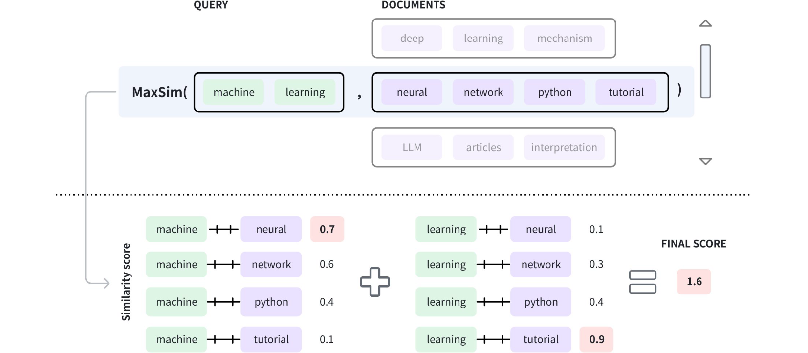
在上述流程中:
-
查询包含两个 Token:
machinelearning
-
文档窗口中包含四个 Token:
neuralnetworkpythontutorial
这些 Token 被向量化后,会计算每个查询 Token 与文档 Token 的相似度,并得到一个相似度分数列表。
然后:
- 从每个查询 Token 对应的相似度列表中选择最高分;
- 将这些最高分进行求和;
- 得到最终文档评分。
该过程称为 最大相似度(Maximum Similarity,MAX_SIM)。
在 Milvus 中实现类似 ColBERT 的文本检索系统时,并不限制只能将文档切分为 Token。
实际上,可以:
- 将文档切分为任意合适大小的 Segment;
- 对每个 Segment 生成 Embedding;
- 创建一个 Embedding List;
- 将文档以及其 Embedding Segment 存储在同一个实体中。
基于 ColBERT,ColPali: Efficient Document Retrieval with Vision Language Models 提出了一种利用视觉语言模型(Vision-Language Model,VLM)的视觉丰富文档检索方法。
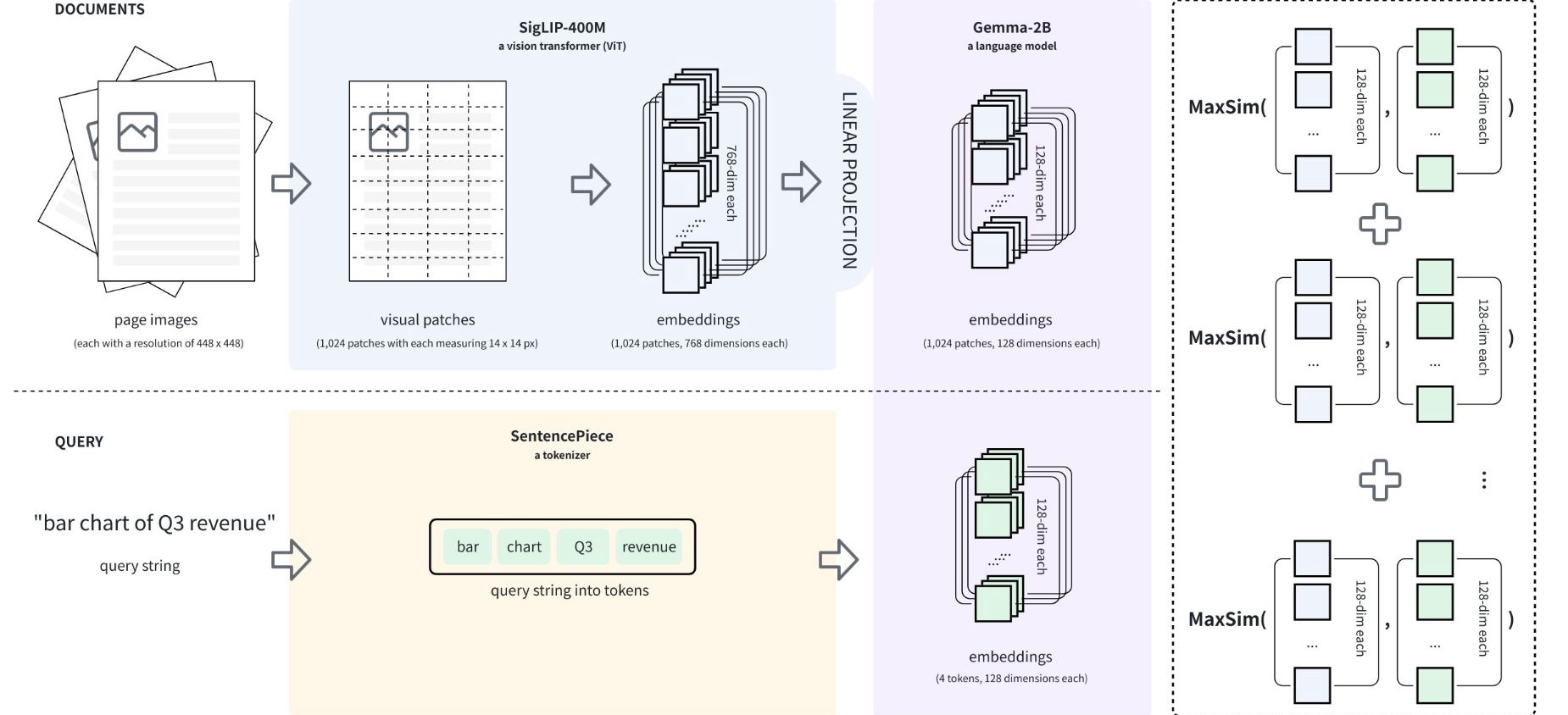
在数据导入阶段:
- 每个文档页面会被渲染为高分辨率图片;
- 图片会被切分为多个 Patch,而不是进行 Token 化。
例如一个:
448 × 448像素的文档页面图片,可以生成:
1024 个 Patch每个 Patch 大小为:
14 × 14像素,这种方式能够保留文本检索系统通常会丢失的非文本信息,例如:
- 文档布局;
- 图片;
- 表格结构。
ColPali 使用的视觉语言模型称为:PaliGemma
该模型由以下部分组成:
- 图像编码器(Image Encoder):SigLIP-400M;
- Decoder-only 语言模型:Gemma2-2B;
- 一个线性层,用于将图像编码器输出映射到语言模型的向量空间。
在数据导入阶段,文档页面以原始图片形式表示,然后:
- 图片被划分为多个视觉 Patch;
- 每个 Patch 被转换为向量;
- 各 Patch Embedding 被映射到语言模型向量空间;
- 得到最终 Embedding List。
表示为:

当查询到达时:
- 查询文本被 Token 化;
- 每个 Token 被转换为向量;
- 生成查询 Embedding List:

随后使用 MAX_SIM 比较两个 Embedding List,并计算查询与文档页面之间的最终相似度分数。
ColBERT 文本检索系统
Step 1:安装依赖
执行以下命令安装所需依赖:
bash
pip install --upgrade huggingface-hub transformers datasets pymilvus cohereStep 2:加载 Cohere 数据集
本示例使用 Cohere 提供的 Wikipedia 数据集,并检索其中前 10,000 条记录。关于该数据集的详细信息,可以参考对应页面。
python
from datasets import load_dataset

lang = "simple"

docs = load_dataset(
    "Cohere/wikipedia-2023-11-embed-multilingual-v3",
    lang,
    split="train[:10000]"
)
执行上述代码后,如果本地不存在该数据集,脚本会自动下载。数据集中每条记录表示 Wikipedia 页面中的一个段落。数据结构如下:
| 字段名称 | 描述 |
|---|---|
_id |
记录 ID |
url |
当前记录对应的 URL |
title |
源文档标题 |
text |
源文档中的一个段落 |
emb |
源文档文本对应的 Embedding |
Step 3:按照标题聚合段落
为了搜索完整文档,而不是单独的段落,需要按照标题对段落进行分组。
python
df = docs.to_pandas()
groups = df.groupby('title')

data = []

for title, group in groups:
    data.append({
        "title": title,
        "paragraphs": [
            {
                "text": row['text'],
                "emb": row['emb']
            }
            for _, row in group.iterrows()
        ]
    })
上述代码中:
- 将按照标题分组后的段落作为完整文档保存;
- 并将结果加入
data列表。
每个文档包含:
python
paragraphs字段。
该字段是一个段落列表。每个段落对象包含:
python
text
emb
两个字段:
text:段落文本;emb:该段落对应的 Embedding。
Step 4:为 Cohere 数据集创建 Collection
准备好数据后,创建 Milvus Collection。该 Collection 中包含一个:
text
paragraphs字段,该字段类型为:
text
Array of Structs代码如下:
python
from pymilvus import MilvusClient, DataType

client = MilvusClient(
    uri="http://localhost:19530",
    token="root:Milvus"
)

# 创建 Collection Schema
schema = client.create_schema()

schema.add_field(
    'id',
    DataType.INT64,
    is_primary=True,
    auto_id=True
)

schema.add_field(
    'title',
    DataType.VARCHAR,
    max_length=512
)


# 创建 Struct Schema
struct_schema = client.create_struct_field_schema()

struct_schema.add_field(
    'text',
    DataType.VARCHAR,
    max_length=65535
)

struct_schema.add_field(
    'emb',
    DataType.FLOAT_VECTOR,
    dim=512
)


schema.add_field(
    'paragraphs',
    DataType.ARRAY,
    element_type=DataType.STRUCT,
    struct_schema=struct_schema,
    max_capacity=200
)


# 创建索引参数
index_params = client.prepare_index_params()

index_params.add_index(
    field_name="paragraphs[emb]",
    index_type="AUTOINDEX",
    metric_type="MAX_SIM_COSINE"
)


# 创建 Collection
client.create_collection(
    collection_name='wiki_documents',
    schema=schema,
    index_params=index_params
)
这里关键点:
paragraphs 是一个结构体数组:
Document
 └── paragraphs[]
      ├── text
      └── emb
每个文档可以包含多个段落,每个段落拥有自己的向量。
索引建立在:
paragraphs[emb]字段上。
使用的距离计算方式:
MAX_SIM_COSINE即 ColBERT 中的最大相似度计算方式。
Step 5:插入 Cohere 数据集
现在可以将准备好的数据插入 Collection:
python
client.insert(
    collection_name='wiki_documents',
    data=data
)
Step 6:搜索 Cohere 数据集
根据 ColBERT 的设计:
查询文本也需要:
- Token 化;
- 转换为 Embedding List。
本步骤使用 Cohere 生成 Wikipedia 数据 Embedding 时使用的同一个模型。
首先调用 Cohere:
python
import cohere

co = cohere.ClientV2("COHERE_API_KEY")
准备查询:
python
query_inputs = [
    {
        'content': [
            {
                'type': 'text',
                'text': 'Adobe'
            },
        ]
    },
    {
        'content': [
            {
                'type': 'text',
                'text': 'software'
            }
        ]
    }
]
生成 Embedding:
python
embeddings = co.embed(
    inputs=query_inputs,
    model='embed-multilingual-v3.0',
    input_type="classification",
    embedding_types=["float"],
)
上述代码中查询文本:
Adobe
software
会被组织成 Token,并转换为一个浮点向量列表。
然后使用 Milvus 的 EmbeddingList 执行搜索:
python
from pymilvus.client.embedding_list import EmbeddingList

query_emb_list = EmbeddingList()

if embeddings.embeddings.float:
    query_emb_list.add_batch(
        embeddings.embeddings.float
    )


results = client.search(
    collection_name="wiki_documents",
    data=[query_emb_list],
    anns_field="paragraphs[emb]",
    search_params={
        "metric_type": "MAX_SIM_COSINE"
    },
    limit=10,
    output_fields=["title"]
)


for hit in results[0]:
    print(
        f"Document {hit['entity']['title']}: {hit['distance']:.4f}"
    )
输出类似:
text
Document Software: 2.3035
Document Application: 2.1875
Document Adobe Illustrator: 2.1167
Document Open source: 2.0542
Document Computer: 1.9811
Document Microsoft: 1.9784
Document Web browser: 1.9655
Document Program: 1.9627
Document Website: 1.9594
Document Computer science: 1.9460
余弦相似度通常范围为:
\[-1,1
]
而上述结果中的相似度分数明显体现了:
最终得分并不是单个向量之间的相似度,而是多个 Token 级相似度分数累加后的结果。
这正是 ColBERT Late Interaction(延迟交互) 的核心思想:
Query Token Embeddings
          |
          v
与 Document Token Embeddings 逐个计算相似度
          |
          v
每个 Query Token 选择最大相似度
          |
          v
所有最大值求和
          |
          v
最终文档评分明白,重新按技术文档翻译格式处理:
- 保留原文标题层级;
- 保留段落结构;
- 表格不拆;
- 代码保持原样,只翻译必要注释;
- 不额外扩展成教程;
- 不使用"一句话一行"的碎片化排版。
ColPali 文本检索系统
Step 1:安装依赖
执行以下命令安装依赖:
bash
pip install --upgrade huggingface-hub transformers datasets pymilvus 'colpali-engine>=0.3.0,<0.4.0'Step 2:加载 Vidore 数据集
本节使用一个名为 vidore_v2_finance_en 的 Vidore 数据集。
该数据集是一个银行领域年度报告语料库,主要用于长文档理解任务。它也是 ViDoRe v3 Benchmark 中包含的 10 个语料库之一。
关于该数据集的详细信息,可以参考对应页面。
python
from datasets import load_dataset

ds = load_dataset("vidore/vidore_v3_finance_en", "corpus")
df = ds['test'].to_pandas()
如果本地不存在该数据集,执行上述代码会自动下载。
数据集中每条记录代表金融报告中的一个页面。
该数据集的结构如下:
| 字段名称 | 描述 |
|---|---|
| corpus_id | 语料库中的一条记录 |
| image | 页面图片的字节数据 |
| doc_id | 描述性文档 ID |
| page_number_in_doc | 当前页面在文档中的页码 |
Step 3:为页面图片生成 Embedding
如 Overview 部分所述,ColPali 模型是一种视觉语言模型(VLM),它可以将图片映射到文本模型的向量空间。
本步骤使用最新的 ColPali 模型:
vidore/colpali-v1.3关于该模型的详细信息,可以参考对应页面。
python
import torch
from typing import cast
from colpali_engine.models import ColPali, ColPaliProcessor

model_name = "vidore/colpali-v1.3"

model = ColPali.from_pretrained(
    model_name,
    torch_dtype=torch.bfloat16,
    device_map="cuda:0",  # 如果使用 Apple Silicon,则设置为 "mps"
).eval()

processor = ColPaliProcessor.from_pretrained(model_name)
模型准备完成后,可以尝试为指定图片生成 Patch:
python
from PIL import Image
from io import BytesIO

# 使用 iterrow() 生成器获取第一行数据
row = next(df.iterrows())[1]

# 将上述行中的图片加入列表
images = [Image.open(BytesIO(row['image']['bytes']))]

patches = processor.process_images(images).to(model.device)
patches_embeddings = model(**patches)[0]

# 查看生成的 Patch Embedding 形状
print(patches_embeddings.shape)

# [1031, 128]
在上述代码中,ColPali 模型会先将图片调整为 448 x 448 像素,然后将其划分为多个 Patch,每个 Patch 的大小为 14 x 14 像素。
最后,这些 Patch 会被转换为 1,031 个 Embedding,每个 Embedding 的维度为 128。
你可以通过循环方式为所有图片生成 Embedding:
python
data = []

for index, row in df.iterrows():
  row = next(df.iterrows())[1]
  corpus_id = row['corpus_id']

  images = [Image.open(BytesIO(row['image']['bytes']))]
  batch_images = processor.process_images(images).to(model.device)
  patches = model(**batch_images)[0]

  doc_id = row['doc_id']
  markdown = row['markdown']
  page_number_in_doc = row['page_number_in_doc']

  data.append({
      "corpus_id": corpus_id,
      "patches": [{"emb": emb} for emb in patches],
      "doc_id": markdown,
      "page_number_in_doc": row['page_number_in_doc']
  })
由于需要处理大量数据并生成 Embedding,因此该步骤耗时相对较长。
Step 4:为金融报告数据集创建 Collection
数据准备完成后,创建 Collection。
其中,名为 patches 的字段是一个 Array of Structs。
python
from pymilvus import MilvusClient, DataType

client = MilvusClient(
    uri=YOUR_CLUSTER_ENDPOINT,
    token=YOUR_API_KEY
)

schema = client.create_schema()

schema.add_field(
    field_name="corpus_id",
    datatype=DataType.INT64,
    is_primary=True
)

patch_schema = client.create_struct_field_schema()

patch_schema.add_field(
    field_name="emb",
    datatype=DataType.FLOAT_VECTOR,
    dim=128
)

schema.add_field(
    field_name="patches",
    datatype=DataType.ARRAY,
    element_type=DataType.STRUCT,
    struct_schema=patch_schema,
    max_capacity=1031
)

schema.add_field(
    field_name="doc_id",
    datatype=DataType.VARCHAR,
    max_length=512
)

schema.add_field(
    field_name="page_number_in_doc",
    datatype=DataType.INT64
)

index_params = client.prepare_index_params()

index_params.add_index(
    field_name="patches[emb]",
    index_type="AUTOINDEX",
    metric_type="MAX_SIM_COSINE"
)

client.create_collection(
    collection_name="financial_reports",
    schema=schema,
    index_params=index_params
)
Step 5:将金融报告插入 Collection
现在可以将准备好的金融报告数据插入创建好的 Collection:
python
client.insert(
    collection_name="financial_reports",
    data=data
)
从输出结果可以看到,Vidore 数据集中的所有页面都已经被插入。
Step 6:在金融报告中进行搜索
数据准备完成后,可以按照如下方式对 Collection 中的数据执行搜索:
python
from pymilvus.client.embedding_list import EmbeddingList

queries = [
    "quarterly revenue growth chart"
]

batch_queries = processor.process_queries(queries).to(model.device)

with torch.no_grad():
    query_embeddings = model(**batch_queries)

query_emb_list = EmbeddingList()
query_emb_list.add_batch(query_embeddings[0].cpu())

results = client.search(
    collection_name="financial_reports",
    data=[query_emb_list],
    anns_field="patches[emb]",
    search_params={
        "metric_type": "MAX_SIM_COSINE"
    },
    limit=10,
    output_fields=["doc_id", "page_number_in_doc"]
)
和普通向量搜索的区别
简单来说:
Embedding List 搜索本质上仍然属于向量搜索,只不过普通向量搜索是一条数据对应一个向量,而 Embedding List 搜索是一条数据对应多个向量,然后通过特殊的聚合方式计算最终相似度。
两者最大的区别在于向量粒度不同:
普通向量搜索:
text
Document
    |
    v
[一个向量]
    |
    v
cosine similarity
    |
    v
score
Embedding List 搜索:
text
Document
    |
    v
[向量1, 向量2, 向量3, ...]
    |
    v
token/patch级别比较
    |
    v
MAX_SIM 聚合
    |
    v
score
我们之前学习 Milvus ANN 时,大部分场景都是这种模式。
例如,一个文档:
text
doc1:
机器学习是一种人工智能技术
经过 embedding 模型编码:
text
doc1

↓

[0.12, 0.54, 0.33, ...]
最终得到一个固定维度的向量,例如:
text
768维向量存储结构类似:
| id | text | vector |
|---|---|---|
| 1 | 机器学习是一种人工智能技术 | 0.12,0.54,... |
用户搜索:
text
什么是机器学习?首先将 query 转换为向量:
text
[0.11,0.52,...]然后计算:
text
query_vector

vs

doc_vector
通过 cosine similarity 等距离函数得到相似度:
text
doc1 score=0.92这就是传统的 Dense Vector Search。
普通向量搜索的问题在于:
一个文档最终只保留了一个向量。
对于短文本,这通常没有问题。但是对于长文档,例如一篇 100 页的报告:
text
第1页:公司介绍

第50页:财务数据

第100页:风险说明
如果直接对整个文档进行 embedding:
text
整个文档

↓

一个768维向量
那么大量细节会被压缩,例如搜索:
text
2024年利润增长多少?整个报告的 embedding 可能更关注:
text
银行
金融
年度报告
公司
而不是:
text
利润增长12%因为单个向量需要表达整个文档的信息,细粒度内容容易丢失。
Embedding List 的核心思想是:
不要把整个文档压缩成一个向量,而是保留多个局部向量。
即,普通方式:
text
document

↓

一个 vector
Embedding List:
text
document

↓

多个 token/chunk/patch

↓

多个 vector
例如一句文本:
text
Machine learning improves security detection可以拆成多个 token:
text
Machine
learning
improves
security
detection然后分别生成 embedding:
text
[
 vector(machine),
 vector(learning),
 vector(improves),
 vector(security),
 vector(detection)
]
这个向量集合就是:
text
Embedding List也就是:
text
[
 e1,
 e2,
 e3,
 e4,
 e5
]
Embedding List 搜索有什么不同?
普通向量搜索中query:
text
machine learning会被编码成一个 query vector:
text
query_vector然后:
text
query_vector

        VS

document_vector
直接计算一次相似度。而 ColBERT 的方式不同。
query:
text
machine learning首先拆成 token:
text
machine
learning得到:
text
[
q1,
q2
]
document:
text
neural network python tutorial得到:
text
[
d1,
d2,
d3,
d4
]
然后进行 token 级别交互。例如:
text
machine

    neural       0.2
    network      0.3
    python       0.1
    tutorial     0.4


learning

    neural       0.5
    network      0.2
    python       0.1
    tutorial     0.3
对于每个 query token,找到 document 中最相似的 token:
text
machine   -> 0.4

learning  -> 0.5
最后求和:
text
score = 0.4 + 0.5这个过程就是:
text
MAX_SIM为什么叫 Late Interaction?
因为它和普通 embedding 最大区别在于:
普通 embedding在生成阶段就完成信息融合:
text
machine learning

        ↓

一个vector
大量语义信息已经压缩到一起。而 ColBERT生成阶段保持 token 独立:
text
machine  -> vector1

learning -> vector2
真正的交互发生在搜索阶段:
text
query token vector

        VS

document token vector
因此称为:
Late Interaction(延迟交互)
总结,
| 普通向量搜索 | Embedding List 搜索 | |
|---|---|---|
| 数据表示 | 一个文档一个 vector | 一个文档多个 vector |
| 检索粒度 | 文档级 | token/patch级 |
| 典型模型 | BERT embedding 等 | ColBERT / ColPali |
| 相似度计算 | vector vs vector | 多个 vector 之间交互 |
| 评分方式 | cosine/IP | MAX_SIM |
| 优势 | 简单、高效 | 保留更多细粒度信息 |
| 缺点 | 可能丢失细节 | 计算和存储成本更高 |
所以:
Embedding List Search 可以理解为:把一个文档拆成多个局部向量并存储在 Milvus 中,在搜索时进行 token/patch 级别的向量匹配。它不是替代普通向量搜索,而是解决"一个文档一个向量导致信息压缩过度"的问题。
前面学习的 ANN、HNSW、IVF、BM25、Hybrid Search,到这里其实正好串起来:
- ANN:解决如何快速找到相似向量;
- BM25:解决关键词相关性排序;
- Hybrid Search:融合稀疏检索和稠密检索;
- ColBERT / ColPali:解决单向量 embedding 表达能力不足的问题。
Search Iterator(搜索迭代器)
ANN Search(近似最近邻搜索)对于单次查询能够召回的实体数量存在最大限制,而简单使用基础 ANN Search 可能无法满足大规模检索场景的需求。
对于 topK 大于 16,384 的 ANN Search 请求,建议考虑使用 SearchIterator(搜索迭代器)。
一次普通的 Search 请求会直接返回搜索结果,而 SearchIterator 会返回一个迭代器(iterator)。
之后可以调用该迭代器的 next() 方法,逐步获取搜索结果。
具体来说,SearchIterator 的使用流程如下:
-
创建一个 SearchIterator,并设置:
- 每次搜索请求返回的实体数量;
- 总共需要返回的实体数量。
-
循环调用 SearchIterator 的
next()方法,以分页方式获取搜索结果。 -
当
next()方法返回空结果时,调用迭代器的close()方法结束循环。
下面的代码展示了如何创建 SearchIterator。
python
from pymilvus import connections, Collection

connections.connect(
    uri="http://localhost:19530",
    token="root:Milvus"
)

# 创建 iterator
query_vectors = [
    [
        0.3580376395471989,
        -0.6023495712049978,
        0.18414012509913835,
        -0.26286205330961354,
        0.9029438446296592
    ]
]

collection = Collection("iterator_collection")

iterator = collection.search_iterator(
    data=query_vectors,
    anns_field="vector",
    param={
        "metric_type": "L2",
        "params": {
            "nprobe": 16
        }
    },
    batch_size=50,
    output_fields=["color"],
    limit=20000
)
在上述示例中:
batch_size设置为 50,表示每次搜索返回的实体数量;limit设置为 20,000,表示总共需要返回的实体数量(即 topK)。
也就是说:
总共获取 20000 条结果

每次返回 50 条
创建 SearchIterator 后,可以调用它的 next() 方法,以分页方式获取搜索结果。
示例:
python
results = []

while True:
    result = iterator.next()

    if not result:
        iterator.close()
        break

    for hit in result:
        results.append(hit.to_dict())
上述代码中:
-
创建一个无限循环;
-
在循环中调用:
pythoniterator.next()获取下一批搜索结果;
-
将返回结果保存到
results变量中; -
当
next()返回空结果时:
python
if not result:说明已经没有更多结果,于是调用:
python
iterator.close()关闭迭代器并结束循环。
简单理解:
普通 Search:
请求

↓

一次返回 topK 条结果
例如:
python
limit=10000直接返回 10000 条。
SearchIterator:
请求

↓

创建 iterator

↓

next()
  ↓
  第1页 50条

next()
  ↓
  第2页 50条

next()
  ↓
  第3页 50条

...
适合:
- 超大 topK 查询;
- 大规模数据导出;
- 分页浏览搜索结果;
- 避免一次性返回大量结果造成内存压力。
本质上类似数据库中的:
sql
LIMIT + OFFSET或者:
python
cursor.fetchmany()不过它针对的是 Milvus 的 ANN 向量检索场景。
使用 Partition Key
Partition Key 是一种基于 Partition(分区)的搜索优化方案。
通过指定某个标量字段(Scalar Field)作为 Partition Key,并在搜索时基于该 Partition Key 设置过滤条件,可以将搜索范围缩小到指定的几个 Partition,从而提升搜索效率。
在 Milvus 中,可以使用 Partition 实现数据隔离,并通过限制搜索范围到指定 Partition 来提升搜索性能。
如果选择手动管理 Partition:
- 一个 Collection 中最多可以创建 1024 个 Partition;
- 插入 Entity 时,需要根据特定规则将 Entity 写入对应的 Partition;
- 搜索时,可以通过限制搜索范围到指定 Partition,减少需要扫描的数据量。
例如,你可以按照业务规则创建多个 Partition:
Collection

├── Partition_A
├── Partition_B
└── Partition_C
然后根据数据所属类别,将 Entity 插入不同 Partition 中。搜索时,只需要查询相关 Partition,而不必扫描整个 Collection。
不过,手动管理 Partition 存在一定限制。对于大规模数据隔离场景,1024 个 Partition 可能无法满足需求,同时用户还需要自行维护数据与 Partition 的映射关系。
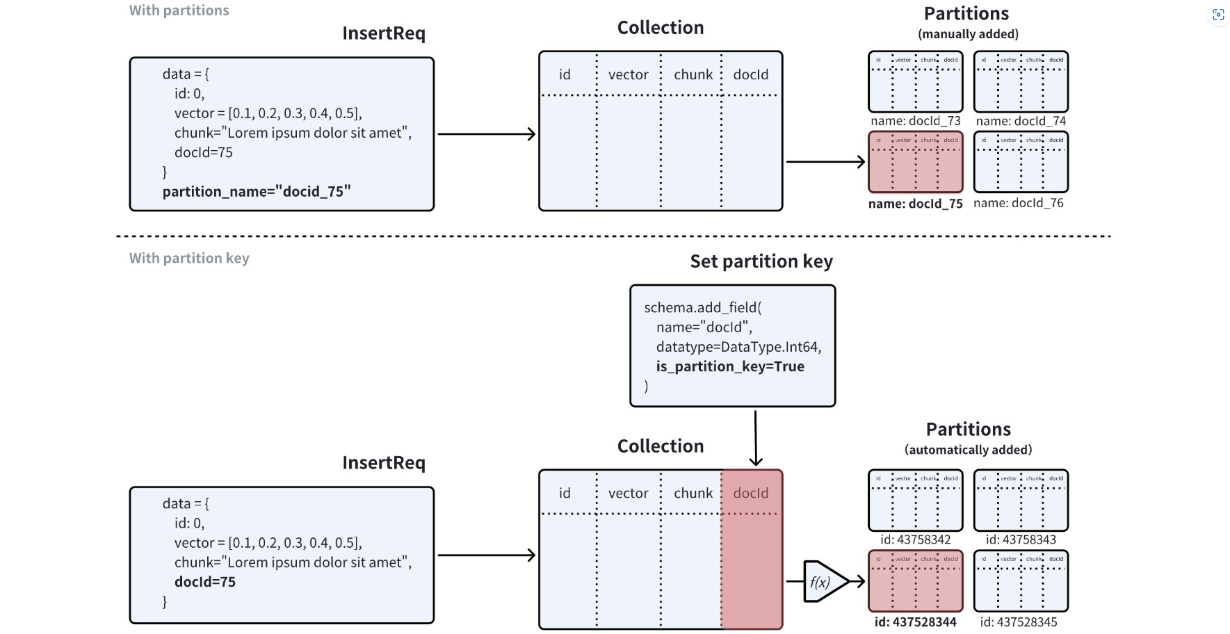
因此,Milvus 引入了 Partition Key,用于解决这一问题。
Partition Key 允许用户在创建 Collection 时,将某个标量字段指定为 Partition Key。
Collection 创建完成后,Milvus 会在 Collection 内部创建指定数量的 Partition。
当插入一个 Entity 时,Milvus 会执行以下流程:
- 获取 Entity 中 Partition Key 字段的值;
- 根据该值计算 Hash 值;
- 使用 Hash 值与 Collection 的
partitions_num属性进行取模计算; - 根据计算结果确定目标 Partition ID;
- 将 Entity 存储到对应 Partition 中。
整个过程如下:
Entity
  |
  v
读取 Partition Key 字段值
  |
  v
计算 Hash
  |
  v
hash % partitions_num
  |
  v
确定目标 Partition
  |
  v
存储 Entity
例如,一个 Entity:
json
{
    "tenant_id": "company_A",
    "vector": [...]
}
如果 tenant_id 被设置为 Partition Key,Milvus 会根据:
hash("company_A") % partitions_num计算该 Entity 应该存储的 Partition。用户不需要手动指定 Partition,Milvus 会自动完成数据分配。
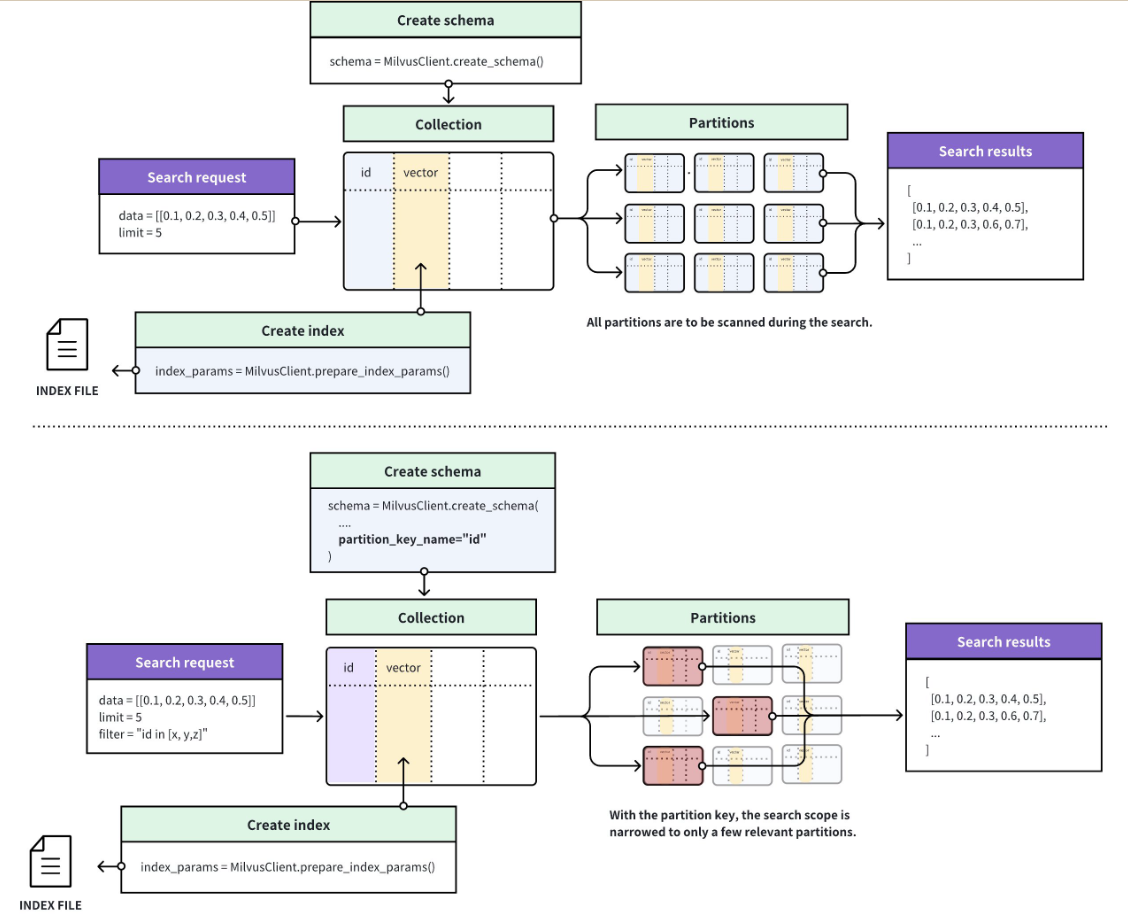
下面展示启用和未启用 Partition Key 时,Milvus 对搜索请求的处理方式。
如果没有启用 Partition Key,Milvus 会在整个 Collection 中搜索与查询向量最相似的 Entity。
流程如下:
Query Vector
      |
      v
整个 Collection
      |
      v
搜索相似 Entity
如果用户知道相关数据位于某个 Partition 中,可以手动指定搜索 Partition,从而缩小搜索范围。
例如:
只搜索 Partition_A这样 Milvus 就不需要扫描其他 Partition。
启用 Partition Key 后,Milvus 会根据搜索请求中的 Partition Key 过滤条件确定搜索范围。
例如:
python
filter = "tenant_id == 'company_A'"Milvus 会根据 Partition Key 的值定位对应 Partition,只搜索匹配 Partition 中的数据。
流程如下:
Query Vector
      +
Partition Key Filter
      |
      v
确定目标 Partition
      |
      v
只搜索目标 Partition
      |
      v
返回结果
因此,相比在整个 Collection 中搜索,Partition Key 可以显著减少需要参与搜索的数据规模。
下面对比没有 Partition Key 和使用 Partition Key 时的搜索过程:
未使用 Partition Key
Collection
├── Partition 1
├── Partition 2
├── Partition 3
└── Partition 4


搜索:
扫描所有 Partition
Milvus 需要在整个 Collection 范围内寻找最相似的数据。
使用 Partition Key
Collection
├── Partition 1
├── Partition 2
├── Partition 3
└── Partition 4


Filter:
tenant_id = "company_A"
        |
        v
定位目标 Partition
        |
        v
只搜索对应 Partition
搜索范围被提前缩小,因此能够提高效率。
要使用 Partition Key,需要完成以下几个步骤:
- 设置 Partition Key;
- 设置需要创建的 Partition 数量(可选);
- 基于 Partition Key 创建过滤条件。
如果想将某个标量字段(Scalar Field)指定为 Partition Key,需要在添加该字段时,将它的 is_partition_key 属性设置为 true。
需要注意的是:
当一个标量字段被设置为 Partition Key 后,该字段的值不能是空值(empty)或
null。
示例:
python
from pymilvus import (
    MilvusClient, DataType
)

client = MilvusClient(
    uri="http://localhost:19530",
    token="root:Milvus"
)

schema = client.create_schema()

schema.add_field(
    field_name="id",
    datatype=DataType.INT64,
    is_primary=True
)

schema.add_field(
    field_name="vector",
    datatype=DataType.FLOAT_VECTOR,
    dim=5
)

# 添加 Partition Key
schema.add_field(
    field_name="my_varchar",
    datatype=DataType.VARCHAR,
    max_length=512,
    is_partition_key=True,
)在上述示例中,my_varchar 字段被设置为了 Partition Key。
当你在 Collection 中指定某个标量字段作为 Partition Key 后,Milvus 默认会自动创建 16 个 Partition。
当 Milvus 接收到一个 Entity 时,会根据该 Entity 的 Partition Key 字段值选择目标 Partition,并将 Entity 存储到对应 Partition 中。
因此,不同 Partition 中可能存储具有不同 Partition Key 值的 Entity。
例如:
Partition Key:

tenant_id
数据:
tenant_id=A
tenant_id=B
tenant_id=C
Milvus 会根据 Hash 结果自动将这些数据分配到不同 Partition。
除了默认的 16 个 Partition 外,你也可以在创建 Collection 时指定 Partition 数量。
注意:
只有在 Collection 中存在被指定为 Partition Key 的标量字段时,
num_partitions参数才有效。
示例:
python
client.create_collection(
    collection_name="my_collection",
    schema=schema,
    num_partitions=128
)
上述代码会创建一个包含 128 个 Partition 的 Collection。
当在启用了 Partition Key 的 Collection 中执行 ANN Search 时,需要在搜索请求中添加一个包含 Partition Key 的过滤表达式(filter expression)。
通过过滤表达式,可以限制 Partition Key 的取值范围,从而让 Milvus 将搜索范围限制在对应的 Partition 内。
例如:
python
filter='partition_key == "x" && <other conditions>'表示:
只搜索 Partition Key 值为 "x" 的数据,同时满足其他过滤条件。
也可以指定多个 Partition Key:
python
filter='partition_key in ["x", "y", "z"] && <other conditions>'表示:
搜索 Partition Key 值属于:
x
y
z
的数据。
在执行删除操作时,建议添加一个指定单个 Partition Key 值的过滤条件。
这样可以让删除操作只作用于某一个 Partition,从而:
- 减少 Compaction(压缩)过程中的写放大(write amplification);
- 降低 Compaction 和索引构建过程中的资源消耗;
- 提升删除效率。
例如:
python
filter='partition_key == "x"'相比:
python
delete all where condition可以避免扫描和处理大量无关 Partition。
需要注意:
示例中的:
python
partition_key只是占位名称。
实际使用时,需要替换成你在 Schema 中设置为 Partition Key 的字段名称。
例如:
如果你的 Partition Key 字段是:
python
tenant_id那么过滤条件应该写成:
python
filter='tenant_id == "company_A"'或者:
python
filter='tenant_id in ["company_A", "company_B"]'这样 Milvus 才能根据 Partition Key 快速定位需要搜索的数据范围。
在多租户(Multi-tenancy)场景中,可以将与租户身份相关的标量字段(Scalar Field)指定为 Partition Key,并基于该字段中的特定值创建过滤条件。
为了进一步提升这类场景下的搜索性能,Milvus 提供了 Partition Key Isolation(Partition Key 隔离) 功能。
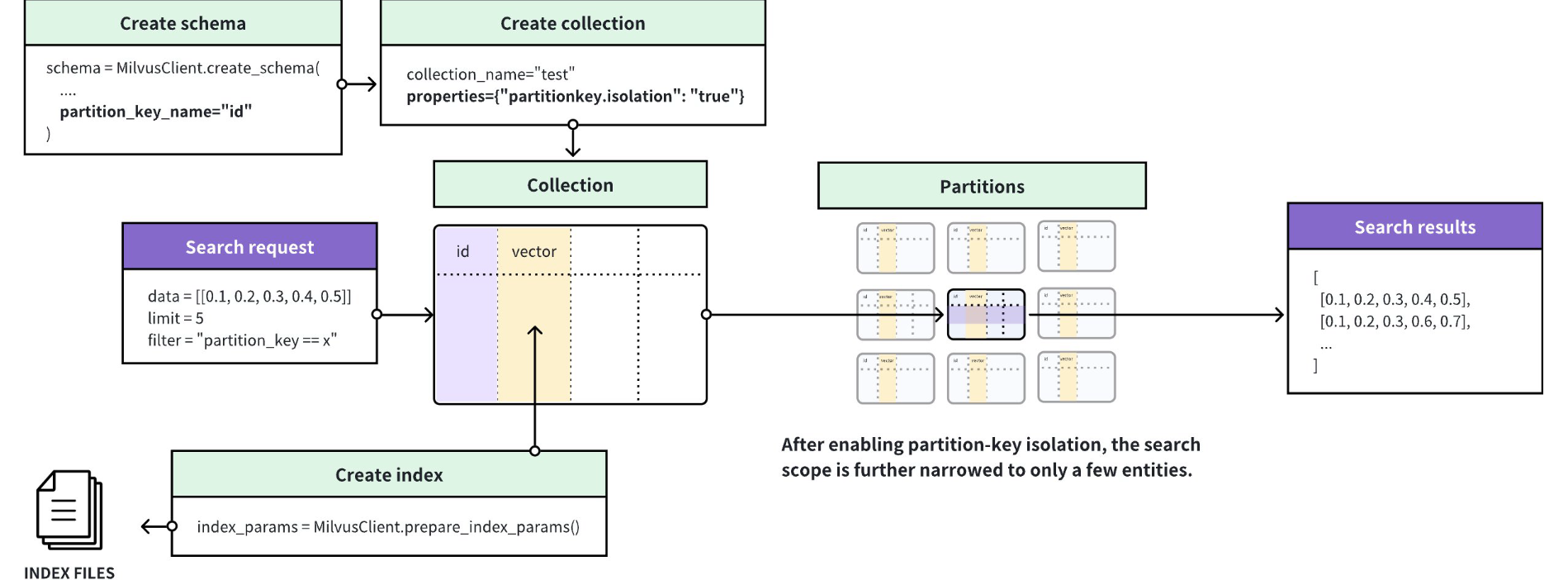
启用 Partition Key Isolation 后,Milvus 会根据 Partition Key 的值对 Entity 进行分组,并为每个分组创建独立的索引。
当 Milvus 接收到搜索请求时,会根据过滤条件中指定的 Partition Key 值定位对应的索引,并将搜索范围限制在该索引包含的 Entity 中。
这样可以避免搜索过程中扫描无关的 Entity,从而显著提升搜索性能。
其流程如下:
Entity

  |
  v

根据 Partition Key 分组

  |
  v

每个分组创建独立索引

  |
  v

搜索请求携带 Partition Key 条件

  |
  v

定位对应索引

  |
  v

只搜索匹配的 Entity
例如,在多租户场景中:
tenant_id = A

    |
    v

Index_A


tenant_id = B

    |
    v

Index_B
搜索:
python
tenant_id == "A"Milvus 会直接使用:
Index_A而不会扫描:
Index_B中的数据。
启用 Partition Key Isolation 后,需要注意:
基于 Partition Key 的过滤条件中必须只包含一个确定的 Partition Key 值,这样 Milvus 才能将搜索范围限制在对应索引中的 Entity。
例如支持:
python
tenant_id == "company_A"因为只有一个确定值。
而:
python
tenant_id in ["company_A", "company_B"]不适用于 Partition Key Isolation,因为它包含多个 Partition Key 值。
目前,Partition Key Isolation 功能仅适用于:
索引类型设置为 HNSW 的搜索场景。
也就是说,只有使用 HNSW 索引时,才能利用 Partition Key Isolation 带来的搜索优化。
下面示例展示如何开启 Partition Key Isolation:
python
client.create_collection(
    collection_name="my_collection",
    schema=schema,
    properties={"partitionkey.isolation": True}
)
启用后,你仍然可以按照前面介绍的方式设置:
- Partition Key;
- Partition 数量。
也就是说:
python
is_partition_key=True以及:
python
num_partitions=128仍然有效。
需要注意:启用 Partition Key Isolation 后,基于 Partition Key 的过滤条件必须只包含一个具体的 Partition Key 值,否则 Milvus 无法利用对应的隔离索引进行搜索优化。
你说得对,这次的问题不是内容,而是我又把整理做成了"分层 PPT 风格",标题、代码块、总结拆得太碎,导致阅读时不断被打断。
你想要的是类似技术博客/源码笔记的整理方式:
- 保留完整上下文;
- 一个主题讲完再进入下一个主题;
- 不要一句话拆成三四行;
- 不要大量"例如:""然后:""所以:"单独占行;
- 代码块只在必要处出现;
- 重点靠段落和小标题组织,而不是靠大量空行。
Milvus Partition Key 机制理解
Partition Key 的思路是:
不要让业务管理 Partition,而是让业务提供一个能够代表数据归属关系的字段。
例如:
python
schema.add_field(
    field_name="tenant_id",
    datatype=DataType.VARCHAR,
    max_length=64,
    is_partition_key=True
)
这里 tenant_id 就是 Partition Key。插入数据:
json
{
    "id": 1,
    "tenant_id": "company_A",
    "text": "xxx",
    "vector": [...]
}
此时用户只需要执行:
python
insert(data)不需要指定:
text
partition_A
partition_B
Milvus 会根据 Partition Key 的值自动计算目标 Partition。
内部过程大致如下:
text
tenant_id = company_A

        ↓

hash(company_A)

        ↓

hash % partitions_num

        ↓

确定目标 Partition
例如:
text
company_A → partition_37那么这条数据会自动写入 partition_37。
因此业务关注:
text
tenant_idMilvus 负责:
text
partition_id很多人会疑惑:
"我不知道 company_A 在 partition_37,那搜索怎么找到?"
实际上搜索时也不需要知道。
例如:
python
filter='tenant_id == "company_A"'Milvus 会根据这个过滤条件重新计算 Partition Key 对应的位置:
text
tenant_id = company_A

        ↓

计算 hash

        ↓

找到对应 Partition

        ↓

只搜索该 Partition
所以用户看到的是:
text
tenant_id而不是:
text
partition_37Partition ID 属于 Milvus 内部实现细节。
Partition Key Isolation 是 Partition Key 的进一步优化。
普通 Partition Key:
text
tenant_id

    ↓

找到 Partition

    ↓

搜索 Partition 中的数据
而 Isolation 会针对不同 Partition Key 值建立独立索引。
例如:
text
tenant_A:

doc1
doc2
doc3


tenant_B:

doc4
doc5
Milvus 可以建立:
text
Index_A

包含 tenant_A 数据


Index_B

包含 tenant_B 数据
搜索:
python
filter='tenant_id=="tenant_A"'可以直接进入:
text
Index_A而不是在一个包含所有租户数据的 HNSW 索引中搜索,再过滤结果。
因此 Isolation 的优化点是:
减少 ANN 搜索范围,避免扫描无关租户的数据。
为什么 Isolation 不支持多个 Partition Key 值?
例如:
python
tenant_id in ["A", "B"]普通 Partition Key 可以处理这种情况。但是 Isolation 的目标是:一次搜索直接定位一个索引。
如果查询:
text
tenant_id in ["A", "B"]那么需要:
text
query

 ├── Index_A
 |
 └── Index_B
同时搜索多个索引。这样就无法发挥 Isolation 的优势。
因此 Partition Key Isolation 要求过滤条件只能指定一个确定的 Partition Key 值。
假设一个企业知识库:
text
tenant_id
project_id
text
vector
有大量租户:
text
tenant_A
tenant_B
tenant_C
...
如果没有 Partition Key:
text
query vector

        ↓

全部租户数据

        ↓

ANN Search
搜索范围非常大。使用 Partition Key:
python
filter='tenant_id=="tenant_A"'Milvus:
text
tenant_A

        ↓

对应 Partition / Index

        ↓

ANN Search
其他租户数据不会参与搜索。
总结:
Partition Key 可以理解为:
用业务字段代替人工管理 Partition。
普通 Partition:
用户告诉 Milvus:"数据放哪个 Partition。"
Partition Key:
用户告诉 Milvus:"数据属于哪个业务实体。"
Milvus 自动决定数据放哪个 Partition。
Partition Key Isolation:
在 Partition Key 的基础上,为不同业务分区建立独立索引,进一步降低搜索范围,提高检索性能。
所以在多租户向量数据库场景中,通常管理的是:
text
tenant_id而不是:
text
partition_37后者只是 Milvus 内部的数据组织方式。
总结
这篇 Milvus 学习到这里,算是告一段落。
从开始学习到现在,累计整理的内容已经超过 100 万字,但即便如此,依然没有覆盖 Milvus 官方文档的全部内容。从这个角度也可以看出,Milvus 本身的体量非常庞大,它已经远远不是一个简单的向量存储组件。
对于一些偏上层的能力,例如内置 Embedding、Rerank 等功能,我暂时将它们作为次级内容处理。原因也很简单:实际工程中完全可以根据业务需求选择合适的 Embedding 模型和 Rerank 模型,通过外部服务调用,而不一定需要强依赖 Milvus 内置实现。未来真正遇到对应场景时,再针对性深入即可。
最开始接触 Milvus,其实只是因为一个很简单的需求:寻找一个比 Faiss 更完整的向量数据库。
Faiss 本身非常优秀,但它更偏向一个高性能向量检索库,主要解决内存中的 ANN 搜索问题,而缺少完整数据库系统需要考虑的数据管理、持久化、分布式、索引管理等能力。因此,当时选择了社区关注度较高的 Milvus,希望了解一个更加工程化的向量数据库方案。
但真正深入之后,Milvus 给我的第一感觉并不是简单,而是复杂。
它更像是在尝试成为一个"面向 AI 时代的综合数据库平台",而不仅仅是一个向量数据库。为了覆盖更多场景,Milvus 引入了大量能力:多种索引类型、标量过滤、文本检索、全文搜索、混合检索、多租户隔离、动态字段、JSON 字段、结构化字段、Embedding List、ColBERT、ColPali 等。
这种设计带来的结果就是:Milvus 的能力非常强,但学习成本也非常高。
尤其是在文本检索部分,仅仅围绕 Search 就存在多种不同方向:
- Text Match;
- Phrase Match;
- Full Text Search;
- BM25;
- Hybrid Search。
这些能力分别对应不同的检索需求,但对于第一次接触的人来说,很容易产生"为什么一个向量数据库需要这么多搜索体系"的疑问。
学习过程中,我也明显感受到 Milvus 中存在很多其他数据库的影子:
- 从 MongoDB 中可以看到灵活字段和文档模型的设计;
- 从 Elasticsearch 中可以看到倒排索引、文本搜索、BM25 等能力;
- 从 ClickHouse 等 OLAP 数据库中可以看到数据组织和查询优化思想;
- 从传统关系数据库中可以看到 Schema、字段类型、索引管理等概念。
某种程度上,Milvus 并不是单纯替代 Faiss,而是在尝试融合传统数据库、搜索引擎以及向量检索系统的能力。
但这也带来了另一个问题:大量复杂度被暴露给了用户。
非常丰富的配置项、庞大的数据类型体系、复杂的索引选择,以及各种高级检索能力,对于研究人员或者需要深度定制检索系统的团队来说非常有价值;但对于普通工程开发者来说,学习曲线确实非常陡峭。
甚至在学习过程中,我第一次遇到一种情况:
一个技术学习完成之后,我依然不确定自己应该如何选择和使用它。
这在之前学习其他组件时并不常见。
通常学习一个数据库、框架或者中间件后,至少能够明确它解决什么问题、什么时候使用。但 Milvus 的问题在于,它覆盖的范围太广,不同场景对应完全不同的能力组合。
最终我对 Milvus 的理解是:
它不是一个简单的"向量数据库",而更像是一个围绕 AI 应用构建的数据基础设施平台。
如果只是简单做向量存储和 ANN 检索,可能只需要掌握:
- Collection;
- Schema;
- Vector Field;
- Index;
- Search。
但如果希望构建企业级知识库、多租户 RAG、复杂检索系统,那么还需要继续深入:
- BM25;
- Hybrid Search;
- Partition Key;
- Rerank;
- ColBERT;
- 多阶段检索;
- 数据隔离与性能优化。
这也是为什么 Milvus 的学习过程会如此漫长。
这篇文章并不是对 Milvus 的否定。相反,正是因为它覆盖了如此多场景,所以才会拥有如此庞大的文档体系。
只是对于工程开发者来说,需要明确自己的目标:
不要试图一次性掌握 Milvus 的全部能力,而应该根据业务场景选择需要的部分。
至此,Milvus 的系统学习暂时告一段落。
后续如果真正进入 RAG、知识库、多模态检索等项目,再结合实际需求继续深入。