datawhale--llm-algo-leetcode0️⃣

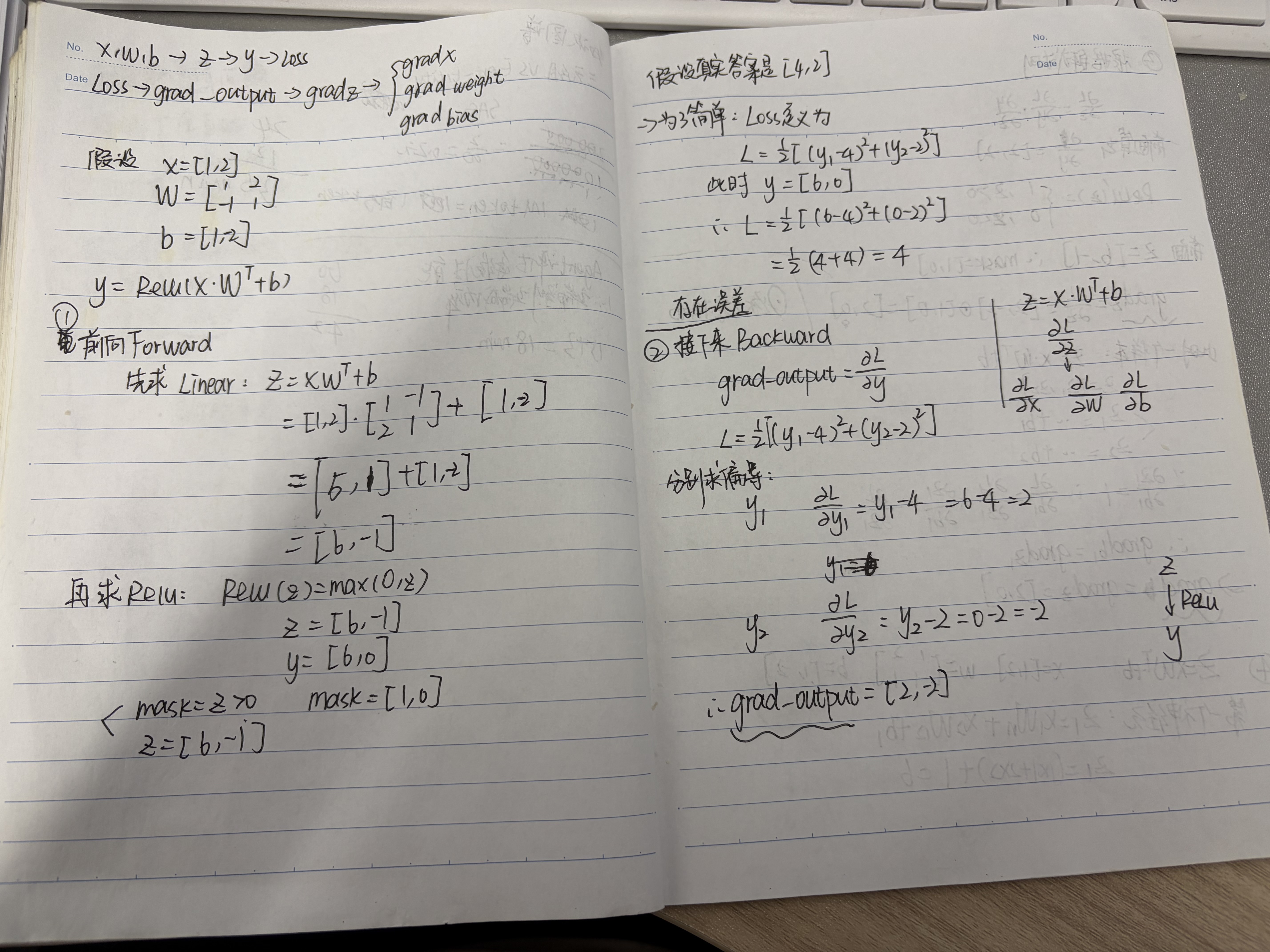
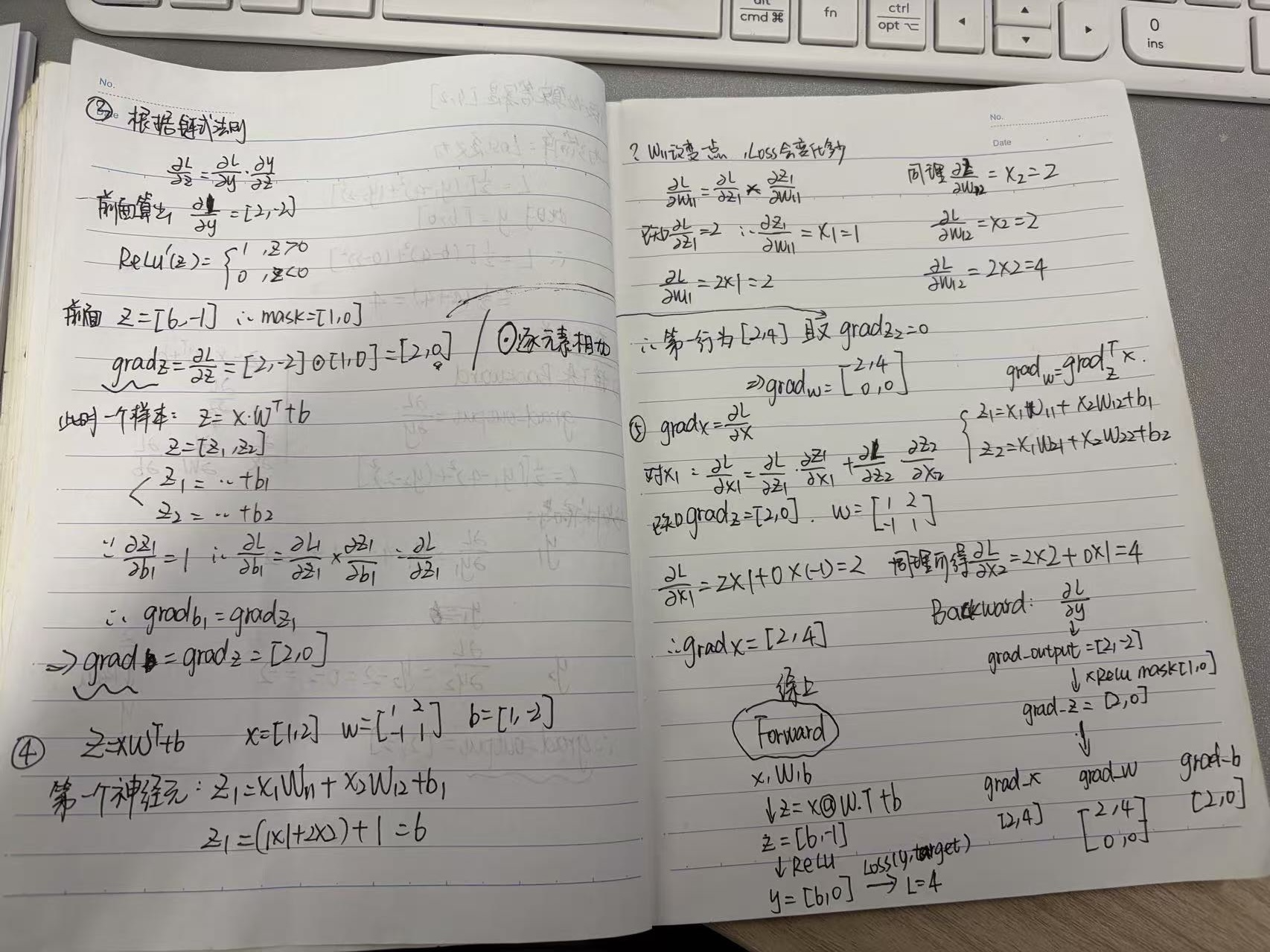
参考链接：笔记地址

0.PyTorch 零基础热身

本页用一个简单问题串起 Python、NumPy、数学和神经网络基础：

给模型一些数据，让它学习规律 y = 2x + 1。

输入 x	输出 y
1	3
2	5
3	7
4	9

Python

名词	简单理解
变量	保存一个值，例如 weight = 2
列表	保存多个值，例如 numbers = [1, 2, 3, 4]
函数	把一段计算封装起来，方便重复调用
循环	对一组数据重复执行相同操作
类	把数据和操作组合成一个对象
模块导入	使用别人已经写好的工具，例如 import numpy as np

weight = 2
bias = 1
numbers = [1, 2, 3, 4]


def calculate(x):
    return weight * x + bias


for number in numbers:
    result = calculate(number)
    print(f"x={number}, y={result}")

输出：

x=1, y=3
x=2, y=5
x=3, y=7
x=4, y=9

神经网络通常会使用类来组织参数和计算过程：

class LinearModel:
    def __init__(self, weight, bias):
        self.weight = weight
        self.bias = bias

    def forward(self, x):
        return self.weight * x + self.bias


model = LinearModel(weight=2, bias=1)
print(model.forward(5))  # 11

NumPy

NumPy 可以方便地处理数组和矩阵：

import numpy as np

x = np.array([
    [1.0],
    [2.0],
    [3.0],
    [4.0],
])

weight = np.array([ [2.0] ])
bias = 1.0

prediction = x @ weight + bias

print("第一行：", x[0])
print("第一列：", x[:, 0])
print("x 的形状：", x.shape)
print("预测结果：\n", prediction)

名词	在示例中的含义
数组	x 是一个形状为 (4, 1) 的二维数组
索引	x[0] 取第一行，x[:, 0] 取第一列
矩阵乘法	x @ weight 将输入与权重相乘
广播	bias 只有一个数，但会自动加到每一行

矩阵形状的变化是：

x           weight       x @ weight
[4, 1]   @  [1, 1]   =   [4, 1]

学习 PyTorch 时，要养成随时查看形状的习惯：

print(x.shape)

数学

名词	通俗理解
向量	一组数字，例如一个学生的 [语文成绩, 数学成绩]
矩阵	多个向量排在一起，例如多个学生的成绩表
导数	参数发生一点变化时，结果会怎样变化
链式法则	一连串计算中，把每一步的影响连接起来

模型的计算公式是：

预测值 = 输入 × 权重 + 偏置
ŷ = xw + b

假设模型预测为 4，真实答案为 5，误差就是：

误差 = 预测值 - 真实值 = 4 - 5 = -1

常用的均方误差损失为：

loss = 平均值((预测值 - 真实值)²)

梯度可以理解为"参数应该往哪个方向修改"。链式法则负责计算一个参数经过多步运算后，最终对损失产生了多大影响。

神经网络

名词	通俗解释
参数	模型需要学习的数字，例如 weight 和 bias
前向传播	使用当前参数，从输入计算出预测值
损失	衡量预测值与真实答案之间的差距
梯度	参数稍微变化时损失会变化多少；正负表示调整方向，绝对值表示影响大小
反向传播	从损失出发，计算每个参数的梯度
梯度下降	根据梯度不断修改参数，让损失逐渐变小

完整流程如下：

输入数据
  ↓
前向传播得到预测值
  ↓
计算损失
  ↓
反向传播计算梯度
  ↓
更新参数
  ↓
重复训练

PyTorch 完整示例

下面让 PyTorch 从 weight = 0、bias = 0 开始，自己学习 y = 2x + 1：

import torch

x = torch.tensor([
    [1.0],
    [2.0],
    [3.0],
    [4.0],
])

y = torch.tensor([
    [3.0],
    [5.0],
    [7.0],
    [9.0],
])

# requires_grad=True 表示需要计算这两个参数的梯度
weight = torch.tensor([[0.0]], requires_grad=True)
bias = torch.tensor(0.0, requires_grad=True)

learning_rate = 0.05

for epoch in range(501):
    # 1. 前向传播
    prediction = x @ weight + bias

    # 2. 计算均方误差损失
    loss = ((prediction - y) ** 2).mean()

    # 3. 反向传播，梯度保存到 weight.grad 和 bias.grad
    loss.backward()

    # 4. 根据梯度更新参数
    with torch.no_grad():
        weight -= learning_rate * weight.grad
        bias -= learning_rate * bias.grad

    # 5. PyTorch 默认会累加梯度，因此每轮训练后需要清零
    weight.grad.zero_()
    bias.grad.zero_()

    if epoch % 100 == 0:
        print(
            f"epoch={epoch}, loss={loss.item():.6f}, "
            f"weight={weight.item():.4f}, bias={bias.item():.4f}"
        )

训练结束后，参数应该接近：

weight = 2
bias = 1

使用学到的参数预测新数据：

new_x = torch.tensor([[5.0]])
prediction = new_x @ weight + bias

print(prediction.item())  # 接近 11

1.张量维度变换与 einops

无论是注意力里的多头合并，还是图像特征、文本特征的整理，都会反复用到张量形状重排。

为什么需要 einops

在大模型开发中，张量形状不匹配，例如 RuntimeError: size mismatch，是非常常见的报错。熟练掌握 PyTorch 原生的 view、reshape、transpose 和 permute 是算法工程师的基础功底。

方法	简单理解
view	在内存布局允许的情况下改变张量形状
reshape	改变张量形状，必要时会创建新的连续数据
transpose	交换两个维度
permute	按指定顺序重新排列多个维度
rearrange	使用有名字的维度描述排列和合并过程

在 Transformer 的多头注意力中，经常需要把张量从：

[batch, heads, seq_len, head_dim]

转换为：

[batch, seq_len, hidden_dim]

其中：

hidden_dim = heads × head_dim

原生 PyTorch 写法

import torch

batch = 2
heads = 4
seq_len = 3
head_dim = 8

x = torch.randn(batch, heads, seq_len, head_dim)

# 第一步：把维度从 [batch, heads, seq_len, head_dim]
# 调整为 [batch, seq_len, heads, head_dim]
x_permuted = x.permute(0, 2, 1, 3)

# 第二步：把 heads 和 head_dim 合并为 hidden_dim
x_native = x_permuted.reshape(batch, seq_len, heads * head_dim)

print("原始形状：", x.shape)
print("调整顺序后：", x_permuted.shape)
print("合并维度后：", x_native.shape)

输出形状：

原始形状：     [2, 4, 3, 8]
调整顺序后：   [2, 3, 4, 8]
合并维度后：   [2, 3, 32]

原生写法可以简写为：

x_native = x.permute(0, 2, 1, 3).reshape(batch, seq_len, -1)

这里的 (0, 2, 1, 3) 分别代表：

0 -> batch
2 -> seq_len
1 -> heads
3 -> head_dim

数字索引虽然简短，但维度较多时容易写错，也不容易看出每个数字的含义。

einops 写法

from einops import rearrange

x_einops = rearrange(x, "b h s d -> b s (h d)")

print(x_einops.shape)

表达式可以这样阅读：

b h s d -> b s (h d)

字母	代表的维度
b	batch，批次大小
h	heads，注意力头数量
s	seq_len，序列长度
d	head_dim，每个注意力头的维度
(h d)	把 heads 和 head_dim 合并成一个维度

与原生写法相比，einops 直接把维度含义写在字符串中，因此代码更容易阅读和维护。

验证两种写法是否一致

print("原生结果形状：", x_native.shape)
print("einops 结果形状：", x_einops.shape)
print("结果是否一致：", torch.equal(x_native, x_einops))

预期输出：

原生结果形状： torch.Size([2, 3, 32])
einops 结果形状： torch.Size([2, 3, 32])
结果是否一致： True

图像特征变成序列

Notebook 中的练习会把图像特征从：

[batch, channels, height, width]

转换为 Transformer 可以处理的序列：

[batch, height × width, channels]

对应代码为：

image = torch.randn(2, 3, 4, 4)

image_native = image.permute(0, 2, 3, 1).reshape(2, 4 * 4, 3)
image_einops = rearrange(image, "b c h w -> b (h w) c")

print(image.shape)          # [2, 3, 4, 4]
print(image_native.shape)   # [2, 16, 3]
print(image_einops.shape)   # [2, 16, 3]
print(torch.equal(image_native, image_einops))  # True

2.Embedding 层：从 Token ID 到连续向量

大模型不能直接理解文字。原始文本需要先经过分词器，例如 BPE，转换成词表中的编号，也就是 token id。Embedding 层再根据这些编号查表，得到模型可以计算的连续向量。

原始文本
  ↓ 分词器
Token
  ↓ 查词表
Token ID
  ↓ Embedding 查表
连续向量
  ↓ Transformer
上下文表示

需要注意：在采用 RoPE 的主流大模型中，RoPE 通常不是直接加到 Embedding 输出上，而是在注意力层中作用于 Query 和 Key，让注意力计算获得位置信息。

Embedding 本质是什么

Embedding 本质上是一张可以训练的二维查找表：

Embedding 表的形状 = [vocab_size, hidden_dim]

名词	含义
vocab_size	词表中一共有多少个 Token
hidden_dim	每个 Token 用多少个数字表示
token id	Token 在词表中的行号
embedding vector	根据 Token ID 取出的那一行向量

例如词表中有 5 个 Token，每个 Token 使用 3 个数字表示：

import torch

embedding_table = torch.tensor([
    [0.1, 0.2, 0.3],  # Token 0
    [0.4, 0.5, 0.6],  # Token 1
    [0.7, 0.8, 0.9],  # Token 2
    [1.0, 1.1, 1.2],  # Token 3
    [1.3, 1.4, 1.5],  # Token 4
])

input_ids = torch.tensor([2, 0, 3])
output = embedding_table[input_ids]

print(output)

输出：

tensor([
    [0.7, 0.8, 0.9],
    [0.1, 0.2, 0.3],
    [1.0, 1.1, 1.2]
])

查表过程就是：

Token ID 2 -> 取第 2 行
Token ID 0 -> 取第 0 行
Token ID 3 -> 取第 3 行

Token ID 只是查表地址，不表示数值大小。Token 100 并不比 Token 5 更重要，也不代表它们在语义上更远。

使用 nn.Embedding

PyTorch 使用 nn.Embedding 创建可以训练的 Embedding 表：

import torch
import torch.nn as nn

torch.manual_seed(42)

vocab_size = 6
hidden_dim = 4

embedding = nn.Embedding(
    num_embeddings=vocab_size,
    embedding_dim=hidden_dim,
)

# 两句话，每句话包含 3 个 Token
# Embedding 的索引必须使用整数类型
input_ids = torch.tensor([
    [1, 4, 2],
    [3, 1, 5],
], dtype=torch.long)

output = embedding(input_ids)

print("词表形状：", embedding.weight.shape)
print("输入形状：", input_ids.shape)
print("输出形状：", output.shape)

预期形状：

词表形状： torch.Size([6, 4])
输入形状： torch.Size([2, 3])
输出形状： torch.Size([2, 3, 4])

形状变化可以理解为：

input_ids: [batch, sequence]
              ↓ 每个 ID 查出一个 hidden_dim 维向量
output:    [batch, sequence, hidden_dim]

在这个例子中：

2 个句子 × 每句 3 个 Token × 每个 Token 4 个数字
= [2, 3, 4]

手动查表与 nn.Embedding 等价

nn.Embedding 的普通查表过程可以手动写成：

output_official = embedding(input_ids)
output_manual = embedding.weight[input_ids]

print(torch.allclose(output_official, output_manual))

预期输出：

True

这说明：

embedding(input_ids)

在直觉上就是：

embedding.weight[input_ids]

embedding_warmup 实现样例

下面的实现与 Notebook 中的函数签名一致。建议先读懂，然后关闭答案，自己重新写一遍。

import torch
import torch.nn as nn


def embedding_warmup(
    input_ids: torch.Tensor,
    vocab_size: int,
    hidden_dim: int,
):
    """比较 nn.Embedding 与手动索引查表的结果。"""

    # 创建形状为 [vocab_size, hidden_dim] 的 Embedding 表
    emb_layer = nn.Embedding(vocab_size, hidden_dim)

    # 固定初始化方式，方便重复实验和比较结果
    with torch.no_grad():
        emb_layer.weight.normal_(mean=0.0, std=0.1)

    # 官方写法：调用 nn.Embedding 进行查表
    out_official = emb_layer(input_ids)

    # 手动写法：直接按照 Token ID 取权重矩阵中的对应行
    out_manual = emb_layer.weight[input_ids]

    return out_official, out_manual

测试代码：

input_ids = torch.tensor(
    [
        [1, 4, 2],
        [3, 0, 5],
    ],
    dtype=torch.long,
)

official, manual = embedding_warmup(
    input_ids=input_ids,
    vocab_size=6,
    hidden_dim=4,
)

print("输入形状：", input_ids.shape)
print("官方输出形状：", official.shape)
print("手动输出形状：", manual.shape)
print("结果是否一致：", torch.allclose(official, manual))

预期输出：

输入形状： torch.Size([2, 3])
官方输出形状： torch.Size([2, 3, 4])
手动输出形状： torch.Size([2, 3, 4])
结果是否一致： True

实现时需要注意：

1. 参数名是 num_embeddings，有复数形式，也可以像示例一样直接传位置参数。
2. 不要在函数内部重新写死 vocab_size 和 hidden_dim，应使用调用者传入的值。
3. input_ids 必须是整数类型，通常使用 torch.long。
4. Token ID 必须满足 0 <= token_id < vocab_size。
5. 官方实现和手动实现必须使用同一张 emb_layer.weight，结果才可以比较。

与 One-hot 加 Linear 的关系

Embedding 在数学上等价于：

1. 把 Token ID 转成 One-hot 向量。
2. 用 One-hot 向量乘以 Embedding 权重矩阵。

import torch.nn.functional as F

one_hot = F.one_hot(
    input_ids,
    num_classes=vocab_size,
).float()

output_one_hot = one_hot @ embedding.weight
output_lookup = embedding(input_ids)

print("One-hot 形状：", one_hot.shape)
print("输出形状：", output_one_hot.shape)
print("结果是否一致：", torch.allclose(output_one_hot, output_lookup))

预期输出：

One-hot 形状： torch.Size([2, 3, 6])
输出形状： torch.Size([2, 3, 4])
结果是否一致： True

矩阵乘法的形状是：

[batch, sequence, vocab_size]
                  @ [vocab_size, hidden_dim]
= [batch, sequence, hidden_dim]

实际模型通常不创建巨大的 One-hot 张量，因为大模型词表可能包含数万甚至更多 Token。直接按照 Token ID 查表更节省内存，计算也更高效。

Embedding 如何学习

Embedding 表中的向量不是人工固定好的，而是模型参数。训练时，反向传播会更新本次使用过的 Token 对应的行。

embedding = nn.Embedding(6, 4)
input_ids = torch.tensor([ [1, 4, 2, 1] ])

output = embedding(input_ids)
loss = (output ** 2).mean()
loss.backward()

gradient = embedding.weight.grad
used_token_ids = torch.where(
    gradient.abs().sum(dim=1) > 0
)[0]

print("本次输入使用的 Token：", input_ids.unique().tolist())
print("获得梯度的词表行：", used_token_ids.tolist())

预期结果中的 Token ID 都是：

[1, 2, 4]

这表示本次前向传播使用了词表中的第 1、2、4 行，所以这些行获得了梯度，并会在参数更新时发生变化。

如何理解 Embedding

可以把 Embedding 想象成一本不断学习的词典：

Token ID -> 词典中的页码
Embedding 表 -> 整本词典
Embedding 向量 -> 对应页面上记录的一组特征

需要记住以下几点：

1. Token ID 只是地址，本身没有连续的数学含义。
2. 同一个 Token ID 在同一个 Embedding 表中会取出相同的初始向量。
3. Embedding 向量会通过反向传播不断更新。
4. 语义相近的 Token 在训练后往往会得到较相近的向量。
5. Embedding 只提供初始表示；经过 Transformer 层后，同一个 Token 在不同上下文中会得到不同的上下文表示。

3. RoPE：旋转位置编码

Embedding 告诉模型"这个 Token 是什么"，但单独的 Embedding 并不知道 Token 出现在句子的第几个位置。

例如下面两句话使用了相同的 Token，但顺序不同：

我 喜欢 猫
猫 喜欢 我

如果只有 Token Embedding，两句话包含的向量集合非常相似。模型还需要位置信息，才能区分不同的排列顺序。

RoPE 的全称是 Rotary Position Embedding，即旋转位置编码。它通过按照 Token 位置旋转 Query 和 Key 的部分维度，把位置信息加入注意力计算。

Embedding 输出
  ↓ 线性投影
Query、Key、Value
  ↓
只对 Query 和 Key 应用 RoPE
  ↓
计算 Attention Score

RoPE 通常不直接修改 Value，也不是简单地把一个位置向量加到 Embedding 上。

二维旋转直觉

先把向量中的两个数字看成二维平面上的一个点：

[x₁, x₂]

将它旋转角度 θ 后得到：

x₁' = x₁ × cos(θ) - x₂ × sin(θ)
x₂' = x₁ × sin(θ) + x₂ × cos(θ)

例如向量 [1, 0] 旋转 90 度后，会接近 [0, 1]。旋转只改变方向，不改变向量长度。

RoPE 会把 head_dim 中的维度两两分组：

(第 0 维, 第 1 维)
(第 2 维, 第 3 维)
(第 4 维, 第 5 维)
...

每一对维度使用不同的旋转速度。同一个 Token 位于不同位置时，旋转角度也不同。

位置越靠后 -> 旋转角度继续累积
不同维度对 -> 使用不同频率

因此，RoPE 要求参与旋转的 head_dim 通常是偶数。

为什么旋转能表示相对位置

假设位置 m 的 Query 旋转了角度 θₘ，位置 n 的 Key 旋转了角度 θₙ。两者进行点积时，最终与角度差有关：

θₙ - θₘ

角度差对应位置差，因此注意力分数可以感知两个 Token 相隔多远。这是 RoPE 非常重要的直觉：

把绝对位置编码成旋转角度，让 Query 和 Key 的点积自然包含相对位置信息。

如何理解 RoPE

可以把 RoPE 想象成给每个位置设置一个不同角度的指针：

Token 内容 -> 由 Embedding 和前面网络层表示
Token 位置 -> 由旋转角度表示
注意力关系 -> Query 与 Key 旋转后的点积

需要记住以下几点：

1. Embedding 负责表示 Token 内容，RoPE 负责让注意力感知位置。
2. RoPE 通常作用于多头注意力中的 Query 和 Key。
3. RoPE 不改变张量形状，也基本不改变向量长度。
4. 不同位置使用不同角度，不同维度对使用不同频率。
5. Query 与 Key 点积时，旋转角度差会体现两个 Token 的相对距离。
6. 这里是便于理解的相邻维度配对实现，真实模型还会加入缓存、缩放和长上下文扩展等工程优化。

4. 前向传播与反向传播

这一节实现一个最小的 Linear + ReLU：

z = x @ weight.T + bias
y = ReLU(z)

假设张量形状为：

x:      [batch, input_dim]
weight: [output_dim, input_dim]
bias:   [output_dim]
y:      [batch, output_dim]

前向传播

精简后的正确实现：

@staticmethod
def forward(ctx, x, weight, bias):
    z = F.linear(x, weight, bias)
    mask = z > 0
    ctx.save_for_backward(x, weight, mask)
    return F.relu(z)

F.linear(x, weight, bias) 等价于：

x @ weight.T + bias

前向传播不仅要计算输出，还要保存反向传播需要的信息：

保存内容	反向传播时的用途
x	计算 weight 的梯度
weight	计算 x 的梯度
mask	判断 ReLU 的哪些位置可以传递梯度

原来的前向写法存在四个问题：

1. weight * x 是逐元素乘法，不是线性层需要的矩阵乘法。
2. relu(z) 没有定义，应使用 F.relu(z)。
3. mask = z 保存的是原始数值，正确 mask 应为 z > 0。
4. 只保存 mask 不够，反向传播还需要 x 和 weight。

反向传播

反向传播接收上游梯度 grad_output，然后按照计算过程反方向传递：

grad_output
  ↓ 经过 ReLU
grad_z
  ↓ 经过 Linear
grad_x、grad_weight、grad_bias

精简实现：

@staticmethod
def backward(ctx, grad_output):
    x, weight, mask = ctx.saved_tensors

    grad_z = grad_output * mask
    grad_x = grad_z @ weight
    grad_weight = grad_z.T @ x
    grad_bias = grad_z.sum(dim=0)

    return grad_x, grad_weight, grad_bias

每个梯度的含义：

梯度	公式	含义
grad_z	grad_output * mask	ReLU 只让 z > 0 的位置传递梯度
grad_x	grad_z @ weight	损失对输入 x 的梯度
grad_weight	grad_z.T @ x	损失对权重的梯度
grad_bias	grad_z.sum(dim=0)	偏置在 batch 中被重复使用，因此要累加

grad_output
=
∂Loss / ∂y

mask
=
∂y / ∂z
=
ReLU 的导数

完整精简版本

class LinearReLUFunction(torch.autograd.Function):
    @staticmethod
    def forward(ctx, x, weight, bias):
        z = F.linear(x, weight, bias)
        mask = z > 0
        ctx.save_for_backward(x, weight, mask)
        return F.relu(z)

    @staticmethod
    def backward(ctx, grad_output):
        x, weight, mask = ctx.saved_tensors
        grad_z = grad_output * mask

        grad_x = grad_z @ weight
        grad_weight = grad_z.T @ x
        grad_bias = grad_z.sum(dim=0)

        return grad_x, grad_weight, grad_bias

学习时建议先只看前向传播，确认每个张量形状；然后关闭答案，自己补全 Notebook 中的 grad_z、grad_x、grad_weight 和 grad_bias。

牢记原则：

Forward：x → z → y → Loss，算预测和误差。

Backward：Loss → y → z → W,b，通过求偏导找到 W、b 应该怎么调整。

5.手搓计算过程（简化版）---便于理解

此部分借助gpt学习推导，有问题感谢🙏留言指教