datawhale--llm-algo-leetcod1️⃣

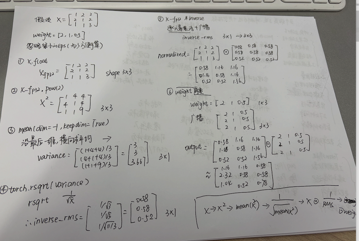
参考链接：笔记

01. RMSNorm 教程笔记

模型架构总览

本节讲解的 RMSNorm 在完整 Transformer 中的位置和数据结构：
#mermaid-svg-2rMdYpI0DUMzgXu6{font-family:"trebuchet ms",verdana,arial,sans-serif;font-size:16px;fill:#333;}@keyframes edge-animation-frame{from{stroke-dashoffset:0;}}@keyframes dash{to{stroke-dashoffset:0;}}#mermaid-svg-2rMdYpI0DUMzgXu6 .edge-animation-slow{stroke-dasharray:9,5!important;stroke-dashoffset:900;animation:dash 50s linear infinite;stroke-linecap:round;}#mermaid-svg-2rMdYpI0DUMzgXu6 .edge-animation-fast{stroke-dasharray:9,5!important;stroke-dashoffset:900;animation:dash 20s linear infinite;stroke-linecap:round;}#mermaid-svg-2rMdYpI0DUMzgXu6 .error-icon{fill:#552222;}#mermaid-svg-2rMdYpI0DUMzgXu6 .error-text{fill:#552222;stroke:#552222;}#mermaid-svg-2rMdYpI0DUMzgXu6 .edge-thickness-normal{stroke-width:1px;}#mermaid-svg-2rMdYpI0DUMzgXu6 .edge-thickness-thick{stroke-width:3.5px;}#mermaid-svg-2rMdYpI0DUMzgXu6 .edge-pattern-solid{stroke-dasharray:0;}#mermaid-svg-2rMdYpI0DUMzgXu6 .edge-thickness-invisible{stroke-width:0;fill:none;}#mermaid-svg-2rMdYpI0DUMzgXu6 .edge-pattern-dashed{stroke-dasharray:3;}#mermaid-svg-2rMdYpI0DUMzgXu6 .edge-pattern-dotted{stroke-dasharray:2;}#mermaid-svg-2rMdYpI0DUMzgXu6 .marker{fill:#333333;stroke:#333333;}#mermaid-svg-2rMdYpI0DUMzgXu6 .marker.cross{stroke:#333333;}#mermaid-svg-2rMdYpI0DUMzgXu6 svg{font-family:"trebuchet ms",verdana,arial,sans-serif;font-size:16px;}#mermaid-svg-2rMdYpI0DUMzgXu6 p{margin:0;}#mermaid-svg-2rMdYpI0DUMzgXu6 .label{font-family:"trebuchet ms",verdana,arial,sans-serif;color:#333;}#mermaid-svg-2rMdYpI0DUMzgXu6 .cluster-label text{fill:#333;}#mermaid-svg-2rMdYpI0DUMzgXu6 .cluster-label span{color:#333;}#mermaid-svg-2rMdYpI0DUMzgXu6 .cluster-label span p{background-color:transparent;}#mermaid-svg-2rMdYpI0DUMzgXu6 .label text,#mermaid-svg-2rMdYpI0DUMzgXu6 span{fill:#333;color:#333;}#mermaid-svg-2rMdYpI0DUMzgXu6 .node rect,#mermaid-svg-2rMdYpI0DUMzgXu6 .node circle,#mermaid-svg-2rMdYpI0DUMzgXu6 .node ellipse,#mermaid-svg-2rMdYpI0DUMzgXu6 .node polygon,#mermaid-svg-2rMdYpI0DUMzgXu6 .node path{fill:#ECECFF;stroke:#9370DB;stroke-width:1px;}#mermaid-svg-2rMdYpI0DUMzgXu6 .rough-node .label text,#mermaid-svg-2rMdYpI0DUMzgXu6 .node .label text,#mermaid-svg-2rMdYpI0DUMzgXu6 .image-shape .label,#mermaid-svg-2rMdYpI0DUMzgXu6 .icon-shape .label{text-anchor:middle;}#mermaid-svg-2rMdYpI0DUMzgXu6 .node .katex path{fill:#000;stroke:#000;stroke-width:1px;}#mermaid-svg-2rMdYpI0DUMzgXu6 .rough-node .label,#mermaid-svg-2rMdYpI0DUMzgXu6 .node .label,#mermaid-svg-2rMdYpI0DUMzgXu6 .image-shape .label,#mermaid-svg-2rMdYpI0DUMzgXu6 .icon-shape .label{text-align:center;}#mermaid-svg-2rMdYpI0DUMzgXu6 .node.clickable{cursor:pointer;}#mermaid-svg-2rMdYpI0DUMzgXu6 .root .anchor path{fill:#333333!important;stroke-width:0;stroke:#333333;}#mermaid-svg-2rMdYpI0DUMzgXu6 .arrowheadPath{fill:#333333;}#mermaid-svg-2rMdYpI0DUMzgXu6 .edgePath .path{stroke:#333333;stroke-width:2.0px;}#mermaid-svg-2rMdYpI0DUMzgXu6 .flowchart-link{stroke:#333333;fill:none;}#mermaid-svg-2rMdYpI0DUMzgXu6 .edgeLabel{background-color:rgba(232,232,232, 0.8);text-align:center;}#mermaid-svg-2rMdYpI0DUMzgXu6 .edgeLabel p{background-color:rgba(232,232,232, 0.8);}#mermaid-svg-2rMdYpI0DUMzgXu6 .edgeLabel rect{opacity:0.5;background-color:rgba(232,232,232, 0.8);fill:rgba(232,232,232, 0.8);}#mermaid-svg-2rMdYpI0DUMzgXu6 .labelBkg{background-color:rgba(232, 232, 232, 0.5);}#mermaid-svg-2rMdYpI0DUMzgXu6 .cluster rect{fill:#ffffde;stroke:#aaaa33;stroke-width:1px;}#mermaid-svg-2rMdYpI0DUMzgXu6 .cluster text{fill:#333;}#mermaid-svg-2rMdYpI0DUMzgXu6 .cluster span{color:#333;}#mermaid-svg-2rMdYpI0DUMzgXu6 div.mermaidTooltip{position:absolute;text-align:center;max-width:200px;padding:2px;font-family:"trebuchet ms",verdana,arial,sans-serif;font-size:12px;background:hsl(80, 100%, 96.2745098039%);border:1px solid #aaaa33;border-radius:2px;pointer-events:none;z-index:100;}#mermaid-svg-2rMdYpI0DUMzgXu6 .flowchartTitleText{text-anchor:middle;font-size:18px;fill:#333;}#mermaid-svg-2rMdYpI0DUMzgXu6 rect.text{fill:none;stroke-width:0;}#mermaid-svg-2rMdYpI0DUMzgXu6 .icon-shape,#mermaid-svg-2rMdYpI0DUMzgXu6 .image-shape{background-color:rgba(232,232,232, 0.8);text-align:center;}#mermaid-svg-2rMdYpI0DUMzgXu6 .icon-shape p,#mermaid-svg-2rMdYpI0DUMzgXu6 .image-shape p{background-color:rgba(232,232,232, 0.8);padding:2px;}#mermaid-svg-2rMdYpI0DUMzgXu6 .icon-shape .label rect,#mermaid-svg-2rMdYpI0DUMzgXu6 .image-shape .label rect{opacity:0.5;background-color:rgba(232,232,232, 0.8);fill:rgba(232,232,232, 0.8);}#mermaid-svg-2rMdYpI0DUMzgXu6 .label-icon{display:inline-block;height:1em;overflow:visible;vertical-align:-0.125em;}#mermaid-svg-2rMdYpI0DUMzgXu6 .node .label-icon path{fill:currentColor;stroke:revert;stroke-width:revert;}#mermaid-svg-2rMdYpI0DUMzgXu6 :root{--mermaid-font-family:"trebuchet ms",verdana,arial,sans-serif;} Transformer Block（Pre-Norm）
残差 x
残差 x'
输入 x

(batch, seq_len, hidden_size)
RMSNorm

Attention 前归一化
Multi-Head Attention
残差连接

x + Attention(...)
中间结果 x'

(batch, seq_len, hidden_size)
RMSNorm

MLP 前归一化
SwiGLU MLP
残差连接

x' + MLP(...)
输出 x''

(batch, seq_len, hidden_size)

本节讲解的模型架构模块

模块	章节	形状变化	核心作用
输入张量	#0.1	[batch, seq_len, hidden_size]	定义数据格式
均方根计算	#2, #6	[batch, seq_len, 1]	计算特征尺度
归一化层	#3-#7	[batch, seq_len, hidden_size]	控制特征尺度
可学习权重	#3, #8	[hidden_size] → 广播	缩放每个特征维度
Pre-Norm 结构	#11	形状不变	先归一化，再进入子层

数据流详解

#mermaid-svg-PLeMr2yOsPVq39sl{font-family:"trebuchet ms",verdana,arial,sans-serif;font-size:16px;fill:#333;}@keyframes edge-animation-frame{from{stroke-dashoffset:0;}}@keyframes dash{to{stroke-dashoffset:0;}}#mermaid-svg-PLeMr2yOsPVq39sl .edge-animation-slow{stroke-dasharray:9,5!important;stroke-dashoffset:900;animation:dash 50s linear infinite;stroke-linecap:round;}#mermaid-svg-PLeMr2yOsPVq39sl .edge-animation-fast{stroke-dasharray:9,5!important;stroke-dashoffset:900;animation:dash 20s linear infinite;stroke-linecap:round;}#mermaid-svg-PLeMr2yOsPVq39sl .error-icon{fill:#552222;}#mermaid-svg-PLeMr2yOsPVq39sl .error-text{fill:#552222;stroke:#552222;}#mermaid-svg-PLeMr2yOsPVq39sl .edge-thickness-normal{stroke-width:1px;}#mermaid-svg-PLeMr2yOsPVq39sl .edge-thickness-thick{stroke-width:3.5px;}#mermaid-svg-PLeMr2yOsPVq39sl .edge-pattern-solid{stroke-dasharray:0;}#mermaid-svg-PLeMr2yOsPVq39sl .edge-thickness-invisible{stroke-width:0;fill:none;}#mermaid-svg-PLeMr2yOsPVq39sl .edge-pattern-dashed{stroke-dasharray:3;}#mermaid-svg-PLeMr2yOsPVq39sl .edge-pattern-dotted{stroke-dasharray:2;}#mermaid-svg-PLeMr2yOsPVq39sl .marker{fill:#333333;stroke:#333333;}#mermaid-svg-PLeMr2yOsPVq39sl .marker.cross{stroke:#333333;}#mermaid-svg-PLeMr2yOsPVq39sl svg{font-family:"trebuchet ms",verdana,arial,sans-serif;font-size:16px;}#mermaid-svg-PLeMr2yOsPVq39sl p{margin:0;}#mermaid-svg-PLeMr2yOsPVq39sl .label{font-family:"trebuchet ms",verdana,arial,sans-serif;color:#333;}#mermaid-svg-PLeMr2yOsPVq39sl .cluster-label text{fill:#333;}#mermaid-svg-PLeMr2yOsPVq39sl .cluster-label span{color:#333;}#mermaid-svg-PLeMr2yOsPVq39sl .cluster-label span p{background-color:transparent;}#mermaid-svg-PLeMr2yOsPVq39sl .label text,#mermaid-svg-PLeMr2yOsPVq39sl span{fill:#333;color:#333;}#mermaid-svg-PLeMr2yOsPVq39sl .node rect,#mermaid-svg-PLeMr2yOsPVq39sl .node circle,#mermaid-svg-PLeMr2yOsPVq39sl .node ellipse,#mermaid-svg-PLeMr2yOsPVq39sl .node polygon,#mermaid-svg-PLeMr2yOsPVq39sl .node path{fill:#ECECFF;stroke:#9370DB;stroke-width:1px;}#mermaid-svg-PLeMr2yOsPVq39sl .rough-node .label text,#mermaid-svg-PLeMr2yOsPVq39sl .node .label text,#mermaid-svg-PLeMr2yOsPVq39sl .image-shape .label,#mermaid-svg-PLeMr2yOsPVq39sl .icon-shape .label{text-anchor:middle;}#mermaid-svg-PLeMr2yOsPVq39sl .node .katex path{fill:#000;stroke:#000;stroke-width:1px;}#mermaid-svg-PLeMr2yOsPVq39sl .rough-node .label,#mermaid-svg-PLeMr2yOsPVq39sl .node .label,#mermaid-svg-PLeMr2yOsPVq39sl .image-shape .label,#mermaid-svg-PLeMr2yOsPVq39sl .icon-shape .label{text-align:center;}#mermaid-svg-PLeMr2yOsPVq39sl .node.clickable{cursor:pointer;}#mermaid-svg-PLeMr2yOsPVq39sl .root .anchor path{fill:#333333!important;stroke-width:0;stroke:#333333;}#mermaid-svg-PLeMr2yOsPVq39sl .arrowheadPath{fill:#333333;}#mermaid-svg-PLeMr2yOsPVq39sl .edgePath .path{stroke:#333333;stroke-width:2.0px;}#mermaid-svg-PLeMr2yOsPVq39sl .flowchart-link{stroke:#333333;fill:none;}#mermaid-svg-PLeMr2yOsPVq39sl .edgeLabel{background-color:rgba(232,232,232, 0.8);text-align:center;}#mermaid-svg-PLeMr2yOsPVq39sl .edgeLabel p{background-color:rgba(232,232,232, 0.8);}#mermaid-svg-PLeMr2yOsPVq39sl .edgeLabel rect{opacity:0.5;background-color:rgba(232,232,232, 0.8);fill:rgba(232,232,232, 0.8);}#mermaid-svg-PLeMr2yOsPVq39sl .labelBkg{background-color:rgba(232, 232, 232, 0.5);}#mermaid-svg-PLeMr2yOsPVq39sl .cluster rect{fill:#ffffde;stroke:#aaaa33;stroke-width:1px;}#mermaid-svg-PLeMr2yOsPVq39sl .cluster text{fill:#333;}#mermaid-svg-PLeMr2yOsPVq39sl .cluster span{color:#333;}#mermaid-svg-PLeMr2yOsPVq39sl div.mermaidTooltip{position:absolute;text-align:center;max-width:200px;padding:2px;font-family:"trebuchet ms",verdana,arial,sans-serif;font-size:12px;background:hsl(80, 100%, 96.2745098039%);border:1px solid #aaaa33;border-radius:2px;pointer-events:none;z-index:100;}#mermaid-svg-PLeMr2yOsPVq39sl .flowchartTitleText{text-anchor:middle;font-size:18px;fill:#333;}#mermaid-svg-PLeMr2yOsPVq39sl rect.text{fill:none;stroke-width:0;}#mermaid-svg-PLeMr2yOsPVq39sl .icon-shape,#mermaid-svg-PLeMr2yOsPVq39sl .image-shape{background-color:rgba(232,232,232, 0.8);text-align:center;}#mermaid-svg-PLeMr2yOsPVq39sl .icon-shape p,#mermaid-svg-PLeMr2yOsPVq39sl .image-shape p{background-color:rgba(232,232,232, 0.8);padding:2px;}#mermaid-svg-PLeMr2yOsPVq39sl .icon-shape .label rect,#mermaid-svg-PLeMr2yOsPVq39sl .image-shape .label rect{opacity:0.5;background-color:rgba(232,232,232, 0.8);fill:rgba(232,232,232, 0.8);}#mermaid-svg-PLeMr2yOsPVq39sl .label-icon{display:inline-block;height:1em;overflow:visible;vertical-align:-0.125em;}#mermaid-svg-PLeMr2yOsPVq39sl .node .label-icon path{fill:currentColor;stroke:revert;stroke-width:revert;}#mermaid-svg-PLeMr2yOsPVq39sl :root{--mermaid-font-family:"trebuchet ms",verdana,arial,sans-serif;} 输入 x

(2, 16, 512)

dtype=FP16
提升到 FP32

(2, 16, 512)
计算均方值

mean(x², dim=-1)

(2, 16, 1)
归一化

x × rsqrt(mean(x²) + eps)

(2, 16, 512)
乘可学习 weight

weight: (512)

(2, 16, 512)
恢复输入精度

FP32 → FP16
输出 y

(2, 16, 512)

关键形状变化总结

步骤	操作	输入形状	输出形状	说明
1	提升精度	[2, 16, 512] FP16	[2, 16, 512] FP32	防止平方溢出
2	计算均方值	[2, 16, 512]	[2, 16, 1]	keepdim=True 保留维度
3	乘以 rsqrt	[2, 16, 512] × [2, 16, 1]	[2, 16, 512]	广播机制
4	乘以 weight	[2, 16, 512] × [512]	[2, 16, 512]	weight 广播
5	恢复精度	[2, 16, 512] FP32	[2, 16, 512] FP16	对齐输入精度

---

0. 学习本章前先认识这些名词

不要一开始就背 RMSNorm 公式。建议先快速认识下面这些名词，知道它们大概在解决什么问题，再进入后面的代码实现。

这一部分不要求一次全部记住。第一次阅读时，重点掌握标有"必须先懂"的内容即可。

0.1 张量和形状

名词	英文	简单理解
张量	Tensor	PyTorch 中保存数字的多维数组
形状	Shape	每个维度分别包含多少个元素
批次	Batch	一次送进模型的样本数量
序列	Sequence	一句话中按顺序排列的 Token
隐藏维度	Hidden Size	每个 Token 使用多少个数字表示
隐藏状态	Hidden State	Token 在模型当前层中的向量表示
最后一维	Last Dimension	通常就是 hidden_size 所在的维度

大模型中的隐藏状态通常具有以下形状：

[batch_size, sequence_length, hidden_size]

例如：

[2, 16, 512]

表示：

2 个样本
每个样本有 16 个 Token
每个 Token 使用 512 个数字表示

RMSNorm 不会混合不同 Token，而是分别处理每个 Token 的 512 维向量。因此本章经常使用：

dim=-1

-1 表示最后一个维度，也就是 hidden_size。

0.2 数学名词

名词	英文	简单理解	在 RMSNorm 中的作用
平方	Square	一个数乘以自己，例如 3² = 9	计算每个特征的能量大小
均值	Mean	一组数字的平均值	对所有隐藏特征求平均
均方值	Mean Square	先平方，再求平均	RMSNorm 的核心统计量
平方根	Square Root	平方的逆运算，例如 sqrt(9) = 3	从均方值得到 RMS
均方根	RMS	平方、平均、开平方	衡量向量整体尺度
方差	Variance	数值相对均值的波动程度	LayerNorm 会使用中心化方差
归一化	Normalization	把数值调整到稳定尺度	防止隐藏状态过大或过小
极小值	Epsilon	很小的安全数，例如 1e-6	防止除以零

需要重点区分：

均方值 = mean(x²)
方差   = mean((x - mean(x))²)

RMSNorm 使用的是均方值，不需要先减去均值。

0.3 模型结构名词

名词	英文	简单理解
LayerNorm	Layer Normalization	减去均值，再根据方差调整尺度
RMSNorm	Root Mean Square Normalization	不减均值，只根据均方根调整尺度
缩放参数	Scale / Gamma	归一化后对每个隐藏特征重新缩放
权重	Weight	本章中指可以学习的缩放参数 weight
偏置	Bias	额外加到输出上的参数；RMSNorm 通常不使用
残差连接	Residual Connection	把子层输出加回原输入
Pre-Norm	Pre-Normalization	先归一化，再进入 Attention 或 MLP

RMSNorm（自己通俗理解：把向量的整体大小调成差不多一样，但是不改变方向） 可以先简单记成：

输入向量
  ↓ 控制整体尺度
RMSNorm
  ↓
Attention 或 MLP

0.4 数值精度名词

名词	英文	简单理解	在本章中的意义
数据类型	dtype	张量使用什么格式保存数字	决定精度和数值范围
单精度	FP32	精度和数值范围较高	用于稳定地计算平方和均值
半精度	FP16	占用显存较少，但数值范围较小	大模型训练和推理常用
BF16	BFloat16	显存占用接近 FP16，数值范围更接近 FP32	大模型训练常见格式
混合精度	AMP	在不同计算中组合使用低精度和高精度	兼顾速度、显存和稳定性
溢出	Overflow	计算结果超过当前类型能表示的范围	FP16 平方时可能得到 inf
无穷大	inf	数值大到无法正常表示	继续计算可能产生异常
非数字	NaN	无效计算产生的特殊结果	可能导致训练失败
升精度	Upcasting	临时从 FP16/BF16 转成 FP32	RMSNorm 平方前的重要操作

本章最重要的精度处理是：

FP16/BF16 输入
  ↓ 转成 FP32
计算平方、均值和 rsqrt
  ↓ 转回原 dtype
输出

0.5 PyTorch API 名词

名词或 API	简单理解	本章中的用途
nn.Module	PyTorch 模型和网络层的基础类	用来定义 RMSNorm 类
nn.Parameter	可以被优化器更新的 Tensor	定义可学习的 weight
forward()	描述输入如何变成输出	实现 RMSNorm 前向传播
pow(2)	对每个元素平方	计算 x²
mean()	对指定维度求平均	计算均方值
dim=-1	选择最后一个维度	对 hidden_size 归一化
keepdim=True	求平均后保留长度为 1 的维度	让结果可以与原张量广播
torch.rsqrt()	计算平方根的倒数	计算 1 / sqrt(x)
x.float()	将张量转换为 FP32	避免半精度平方溢出
x.dtype	查看输入的数据类型	最后恢复输出精度
广播	Broadcasting	自动扩展长度为 1 的维度

0.6 先看懂这个最小预习代码

进入 RMSNorm 正文前，先运行下面的代码：

import torch

# 2 个样本，每个样本有 3 个 Token，每个 Token 有 4 个隐藏特征
x = torch.randn(2, 3, 4)

# 统计计算先使用 FP32
x_fp32 = x.float()

# 对最后一个隐藏维度计算均方值
mean_square = x_fp32.pow(2).mean(dim=-1, keepdim=True)

# 计算均方根的倒数
inverse_rms = torch.rsqrt(mean_square + 1e-6)

# 使用广播调整每个 Token 向量的尺度
normalized = x_fp32 * inverse_rms

print("输入形状：", x.shape)
print("均方值形状：", mean_square.shape)
print("归一化结果形状：", normalized.shape)
print("归一化后的均方：\n", normalized.pow(2).mean(dim=-1))

预期形状：

输入形状：       torch.Size([2, 3, 4])
均方值形状：     torch.Size([2, 3, 1])
归一化结果形状： torch.Size([2, 3, 4])

阅读代码时，只需要先回答四个问题：

1. 为什么输入是三维张量？
2. 为什么使用 dim=-1？
3. 为什么需要 keepdim=True？
4. 为什么平方前先执行 x.float()？

能够大概回答这四个问题后，再进入下面的 RMSNorm 正文。

0.7 推荐学习顺序

第一步：认识张量形状和最后一维
  ↓
第二步：理解平方、均值和 RMS
  ↓
第三步：理解广播和 keepdim
  ↓
第四步：理解 FP16、FP32 和溢出
  ↓
第五步：理解 nn.Module 与 nn.Parameter
  ↓
第六步：实现 RMSNorm

RMSNorm 是大模型中常见的归一化层。它的主要作用是控制隐藏状态的数值尺度，让深层网络的训练和推理更加稳定。

本节对应：

02_PyTorch_Algorithms/01_RMSNorm_Tutorial.ipynb

学习目标：

1. 理解为什么神经网络需要归一化。
2. 理解 RMSNorm 与 LayerNorm 的区别。
3. 看懂 RMSNorm 的公式和张量形状。
4. 独立实现一个支持 FP16 的 RMSNorm。
5. 理解 eps、keepdim、rsqrt 和可学习参数 weight 的作用。

1. 为什么需要归一化

Transformer 中的数据会不断经过线性层、Attention、激活函数和残差连接。随着网络层数增加，中间张量的数值尺度可能不断变化。

例如某一层的隐藏状态可能是：

[0.1, 0.2, 0.3]

经过多层计算后，也可能变成：

[100.0, -80.0, 50.0]

如果数值尺度变化太大，可能出现：

• 梯度不稳定。
• 激活值过大或过小。
• FP16 计算溢出。
• 模型难以训练。

归一化层会把每个 Token 的隐藏向量调整到相对稳定的尺度。

可以简单理解为：

归一化不负责改变 Token 表达的主要方向，而是避免向量整体过大或过小。

2. RMS 是什么

RMS 是 Root Mean Square，即均方根。

给定一个向量：

x = [x₁, x₂, ..., x_d]

RMS 的计算过程是：

平方 -> 求平均 -> 开平方

公式为：

RMS(x) = sqrt(mean(x²) + eps)

例如：

x = [3, 4]

计算过程：

平方：       [9, 16]
平均：       (9 + 16) / 2 = 12.5
开平方：     sqrt(12.5) ≈ 3.535

PyTorch 示例：

import torch

x = torch.tensor([3.0, 4.0])
eps = 1e-6

mean_square = x.pow(2).mean()
rms = torch.sqrt(mean_square + eps)
normalized = x / rms

print("均方：", mean_square)
print("RMS：", rms)
print("归一化结果：", normalized)
print("归一化后的均方：", normalized.pow(2).mean())

最后一行结果应该接近：

1.0

这表示归一化后的向量，其平均平方值被调整到了接近 1。

3. RMSNorm 公式

给定输入向量：

x ∈ R^d

RMSNorm 分为两步。

计算均方根

RMS(x) = sqrt(mean(x²) + eps)

其中：

• d 是隐藏维度 hidden_size。
• eps 是一个很小的数，例如 1e-6。
• eps 用于防止输入全为零时发生除零。

归一化并缩放

y = x / RMS(x) × weight

其中 weight 是可学习参数，也可以写作 γ：

weight.shape = [hidden_size]

初始化时通常使用全 1：

self.weight = nn.Parameter(torch.ones(hidden_size))

这样模型刚开始训练时，weight 不会额外改变归一化结果。

4. RMSNorm 与 LayerNorm

LayerNorm 和 RMSNorm 都是在最后一个隐藏维度上做归一化，但计算方式不同。

对比项	LayerNorm	RMSNorm
是否减去均值	是	否
是否计算中心化方差	是	否
是否计算均方值	间接需要	是
可学习缩放参数	有	有
可学习偏置	通常有	通常没有
主要作用	调整均值和尺度	主要调整尺度

LayerNorm 可以简化理解为：

(x - mean(x)) / sqrt(var(x) + eps)

RMSNorm 为：

x / sqrt(mean(x²) + eps)

RMSNorm 不执行减均值操作，因此实现更简单。教程中的直觉是：在大型网络中，重新调整中心位置不一定总是必要，只控制特征尺度也可以保持较好的稳定性。

需要注意：代码中经常把 mean(x²) 命名为 variance，但它严格来说是"均方值"，不是减去均值后的中心化方差。

5. 张量形状

大模型中的隐藏状态通常是三维张量：

x.shape = [batch, sequence, hidden_size]

例如：

x.shape = [2, 16, 512]

表示：

• 2 个样本。
• 每个样本包含 16 个 Token。
• 每个 Token 使用 512 个数字表示。

RMSNorm 对每个 Token 的 hidden_size 维向量独立归一化，因此需要在最后一维计算均方值：

mean_square = x.pow(2).mean(dim=-1, keepdim=True)

形状变化：

x:           [2, 16, 512]
mean_square: [2, 16, 1]

保留最后一个长度为 1 的维度，是为了让 PyTorch 使用广播机制：

[2, 16, 512] × [2, 16, 1]

如果没有 keepdim=True：

mean_square.shape = [2, 16]

它将无法直接按照预期与 [2, 16, 512] 相乘。

6. 为什么使用 torch.rsqrt

根据公式，我们需要计算：

1 / sqrt(mean_square + eps)

PyTorch 可以直接写成：

torch.rsqrt(mean_square + eps)

rsqrt 表示 reciprocal square root，即平方根的倒数：

rsqrt(x) = 1 / sqrt(x)

因此归一化可以写成：

x * torch.rsqrt(mean_square + eps)

它与下面的写法含义相同：

x / torch.sqrt(mean_square + eps)

7. FP16 数值溢出

RMSNorm 的第一步是计算平方：

x.pow(2)

但 FP16 能表示的最大有限数大约是 65504。如果输入中出现 300：

300² = 90000

这个结果超过 FP16 的范围，可能变成 inf，后续计算可能产生 NaN。

示例：

x = torch.tensor([300.0], dtype=torch.float16)
print(x.pow(2))

为了避免平方时溢出，通常先把输入提升到 FP32：

x_fp32 = x.float()
mean_square = x_fp32.pow(2).mean(dim=-1, keepdim=True)

完成归一化后，再把结果转换回输入精度：

output = output.to(x.dtype)

需要形成一个重要的工程习惯：

容易发生溢出的统计计算先使用 FP32，完成后再恢复原始 dtype。

8. 分步骤实现 RMSNorm

第一步：定义可学习参数

self.weight = nn.Parameter(torch.ones(hidden_size))

为什么需要 nn.Parameter：

• 普通 Tensor 不会自动成为模型参数。
• nn.Parameter 会被 model.parameters() 找到。
• 优化器会在训练过程中更新它。

第二步：计算归一化结果

def _norm(self, x: torch.Tensor) -> torch.Tensor:
    x_fp32 = x if x.dtype == torch.float32 else x.float()
    mean_square = x_fp32.pow(2).mean(dim=-1, keepdim=True)
    return x_fp32 * torch.rsqrt(mean_square + self.eps)

这段代码做了三件事：

1. 将输入提升到 FP32。
2. 在最后一个维度计算均方值。
3. 使用均方根的倒数调整输入尺度。

第三步：缩放并恢复精度

def forward(self, x: torch.Tensor) -> torch.Tensor:
    weight = self.weight.to(x.dtype)
    normalized = self._norm(x)
    return (weight * normalized).to(x.dtype)

weight.shape 为：

[hidden_size]

PyTorch 会将它广播到：

[batch, sequence, hidden_size]

9. 完整精简实现

import torch
import torch.nn as nn


class RMSNorm(nn.Module):
    def __init__(self, hidden_size: int, eps: float = 1e-6):
        super().__init__()
        self.eps = eps
        self.weight = nn.Parameter(torch.ones(hidden_size))

    def _norm(self, x: torch.Tensor) -> torch.Tensor:
        x_fp32 = x if x.dtype == torch.float32 else x.float()
        mean_square = x_fp32.pow(2).mean(dim=-1, keepdim=True)
        return x_fp32 * torch.rsqrt(mean_square + self.eps)

    def forward(self, x: torch.Tensor) -> torch.Tensor:
        weight = self.weight.to(x.dtype)
        return (weight * self._norm(x)).to(x.dtype)

实现主线只有四步：

输入转 FP32
  ↓
计算最后一维的 mean(x²)
  ↓
乘以 rsqrt(mean(x²) + eps)
  ↓
乘以 weight 并恢复原 dtype

10.最简单的例子来理解

import torch
import torch.nn as nn

class RMSNorm(nn.Module):
    def __init__(self, hidden_size: int, eps: float = 1e-6):
        super().__init__()
        self.eps = eps

        # 可学习参数，长度等于 hidden_size
        # 一开始全部是 1
        self.weight = nn.Parameter(torch.ones(hidden_size))

    def forward(self, x: torch.Tensor) -> torch.Tensor:
        # x.shape = [batch, seq_len, hidden_size]
        # 这里例子中就是 [1, 3, 3]

        # 临时转成 FP32，避免平方时 FP16 溢出
        x_fp32 = x.float()

        # 对最后一维 hidden_size 求平方后的平均值
        # [1, 3, 3] -> [1, 3, 1]
        mean_square = x_fp32.pow(2).mean(dim=-1, keepdim=True)

        # 计算 1 / sqrt(mean_square + eps)
        # shape 仍然是 [1, 3, 1]
        inverse_rms = torch.rsqrt(mean_square + self.eps)

        # [1, 3, 3] * [1, 3, 1]
        # [1, 3, 1] 会自动广播成 [1, 3, 3]
        # 所以 normalized 最终仍然是 [1, 3, 3]
        normalized = x_fp32 * inverse_rms

        # weight.shape = [3]
        # 会自动广播到每个 token 的 hidden_size
        # 最终 shape 仍然是 [1, 3, 3]
        output = normalized * self.weight

        return output.to(x.dtype)


# ============================================================
# 同一个输入，一次性观察整个 RMSNorm 过程
# ============================================================

x = torch.tensor([
    [
        [1.0, 2.0, 2.0],
        [2.0, 1.0, 2.0],
        [1.0, 1.0, 3.0],
    ]
])

norm = RMSNorm(hidden_size=3)

# 原始输入
print("x:")
print(x)
print("x.shape =", x.shape)

# 平方
x_fp32 = x.float()
x_square = x_fp32.pow(2)

print("\nx²:")
print(x_square)
print("x².shape =", x_square.shape)

# dim=-1：沿最后一维求平均
# [1,3,3] -> [1,3,1]
mean_square = x_square.mean(dim=-1, keepdim=True)

print("\nmean_square:")
print(mean_square)
print("mean_square.shape =", mean_square.shape)

# 计算倒数平方根
inverse_rms = torch.rsqrt(mean_square + 1e-6)

print("\ninverse_rms:")
print(inverse_rms)
print("inverse_rms.shape =", inverse_rms.shape)

# 广播：
# x              [1,3,3]
# inverse_rms    [1,3,1]
#                  ↓
# inverse_rms 会在最后一维复制
# 最终 normalized 仍然是 [1,3,3]
normalized = x_fp32 * inverse_rms

print("\nnormalized:")
print(normalized)
print("normalized.shape =", normalized.shape)

# 当前 RMSNorm 的可学习参数
print("\nweight:")
print(norm.weight)
print("weight.shape =", norm.weight.shape)

# weight=[1,1,1] 时，输出和 normalized 一样
out = norm(x)

print("\nRMSNorm output:")
print(out)
print("output.shape =", out.shape)


# ============================================================
# 手动修改 weight，再观察
# ============================================================

with torch.no_grad():
    norm.weight[:] = torch.tensor([2.0, 1.0, 0.5])

print("\n修改后的 weight:")
print(norm.weight)

out2 = norm(x)

print("\n修改 weight 后的 output:")
print(out2)
print("output.shape =", out2.shape)


# ============================================================
# 对比 dim=-1 和 dim=1
# 注意：这里使用的仍然是完全相同的 x
# ============================================================

dim_last = x.pow(2).mean(dim=-1, keepdim=True)

dim_1 = x.pow(2).mean(dim=1, keepdim=True)

print("\n================ dim 对比 ================")

print("\ndim=-1:")
print(dim_last)
print("shape =", dim_last.shape)
# [1,3,3] -> [1,3,1]
# 每一行的 3 个 hidden 特征被求平均


print("\ndim=1:")
print(dim_1)
print("shape =", dim_1.shape)
# [1,3,3] -> [1,1,3]
# 三行在 seq_len 方向被求平均

输出的结果：

x:
tensor([[[1., 2., 2.],
         [2., 1., 2.],
         [1., 1., 3.]]])
x.shape = torch.Size([1, 3, 3])

x²:
tensor([[[1., 4., 4.],
         [4., 1., 4.],
         [1., 1., 9.]]])
x².shape = torch.Size([1, 3, 3])

mean_square:
tensor([[[3.0000],
         [3.0000],
         [3.6667]]])
mean_square.shape = torch.Size([1, 3, 1])

inverse_rms:
tensor([[[0.5774],
         [0.5774],
         [0.5222]]])
inverse_rms.shape = torch.Size([1, 3, 1])

normalized:
tensor([[[0.5774, 1.1547, 1.1547],
         [1.1547, 0.5774, 1.1547],
         [0.5222, 0.5222, 1.5667]]])
normalized.shape = torch.Size([1, 3, 3])

weight:
Parameter containing:
tensor([1., 1., 1.], requires_grad=True)
weight.shape = torch.Size([3])

RMSNorm output:
tensor([[[0.5774, 1.1547, 1.1547],
         [1.1547, 0.5774, 1.1547],
         [0.5222, 0.5222, 1.5667]]], grad_fn=<MulBackward0>)
output.shape = torch.Size([1, 3, 3])

修改后的 weight:
Parameter containing:
tensor([2.0000, 1.0000, 0.5000], requires_grad=True)

修改 weight 后的 output:
tensor([[[1.1547, 1.1547, 0.5774],
         [2.3094, 0.5774, 0.5774],
         [1.0445, 0.5222, 0.7833]]], grad_fn=<MulBackward0>)
output.shape = torch.Size([1, 3, 3])

================ dim 对比 ================

dim=-1:
tensor([[[3.0000],
         [3.0000],
         [3.6667]]])
shape = torch.Size([1, 3, 1])

dim=1:
tensor([[[2.0000, 2.0000, 5.6667]]])
shape = torch.Size([1, 1, 3])