【流匹配模型Flow Maching】流匹配模型入门理解（3）

目录

• 前言
• [1. 条件流匹配理解](#1. 条件流匹配理解)
• [2. 标签数据导入](#2. 标签数据导入)
• [2. 构造训练路径](#2. 构造训练路径)
• [3. 条件速度预测网络](#3. 条件速度预测网络)
• [4. 条件训练](#4. 条件训练)
• [5. 指定条件，从噪声逐步生成。](#5. 指定条件，从噪声逐步生成。)
• [6. 相同起点和条件，一步与多步比较。](#6. 相同起点和条件，一步与多步比较。)
• [7. 相同噪声，不同条件对比](#7. 相同噪声，不同条件对比)

前言

下面在这个代码的基础上 【流匹配模型Flow Maching】流匹配模型入门理解（2），讲一下条件流模型。

1. 条件流匹配理解

之前的模型是：

v θ ( x t , t ) v_\theta(x_t, t) vθ(xt,t)

现在的条件流模型，最核心的变化就是：

v θ ( x t , t , c ) \boxed{v_\theta(x_t, t, c)} vθ(xt,t,c)

网络根据当前位置 x t x_t xt、时间 t t t，以及条件 c c c，决定接下来往哪里移动、移动多快。也就是说条件流模型是多加了给定条件下当前点的速度是多少。与之对应的数据也得用相应的条件标签，而学习的目标从整体的分布的直接生成，变成了
p d a t a ( x ∣ c ) \boxed{p_{\mathrm{data}}(x \mid c)} pdata(x∣c)
注意：条件决定目标分布，不决定某一个唯一的输出点。也就是说给定条件学习的是整个概率分布而不会考虑概率分布中的点在每次输出中变不变，即固定 (c=0)，换不同的初始噪声，仍应生成第一条月牙上不同的位置。这个地方补充一下数据，之前的数据是两条月牙形的分布，模型生成的是两条月牙的整个分布。在条件流模型中，这个数据改造一下为每个月牙打个标签，一条为1，一条为0，详细见下面的代码。

训练公式几乎不用改，只需要把条件传给网络训练时抽取：

( x 1 , c ) ∼ p d a t a ( x , c ) , z ∼ N ( 0 , I ) , t ∼ U ( 0 , 1 ) (x_1, c) \sim p_{\mathrm{data}}(x, c), \qquad z \sim \mathcal{N}(0, I), \qquad t \sim U(0, 1) (x1,c)∼pdata(x,c),z∼N(0,I),t∼U(0,1)

这里 x 1 x_1 x1 与 c c c 必须对应。例如，第一条月牙上的真实点就必须带第一类标签。噪声仍可以独立抽取。然后：

x t = ( 1 − t ) z + t x 1 x_t = (1 - t) z + t x_1 xt=(1−t)z+tx1

u = x 1 − z u = x_1 - z u=x1−z

条件模型的损失就是：

L ( θ ) = E x 1 , c , z , t ∥ v θ ( x t , t , c ) − ( x 1 − z ) ∥ 2 2 \boxed{\mathcal{L}(\theta) = \mathbb{E}_{x_1, c, z, t} \left \\left\\\| v_\\theta(x_t, t, c) - (x_1 - z) \\right\\\|_2\^2 \\right} L(θ)=Ex1,c,z,t∥vθ(xt,t,c)−(x1−z)∥22

你可能会问："目标速度的公式里没有 c c c，那条件到底起什么作用？"因为条件已经通过训练数据的配对进入目标了：

• 当 c = 0 c = 0 c=0，终点 x 1 x_1 x1 来自第一条月牙。
• 当 c = 1 c = 1 c=1，终点 x 1 x_1 x1 来自第二条月牙。

因此，不同条件下，网络看到的是通向不同目标分布的速度监督。不需要手动在 x_data - noise 里再加一个条件项。个人简单理解，模型训练了在每个条件下的监督信号，当给定这个条件就会生成相应的速度。

为什么加入条件能够改变生成方向？

想象在相同时间 t t t、相同位置 x t x_t xt，网络收到两种输入：

model(x_t, t, c=0)
model(x_t, t, c=1)

它们可以给出不同速度，因为目标分布不同。从平方误差回归的角度，理想网络学到的是：

v ∗ ( x , t , c ) = E x 1 − z ∣ x t = x , t , c \boxed{v^*(x, t, c) = \mathbb{E} \left x_1 - z \\mid x_t = x, \\ t, \\ c \\right} v∗(x,t,c)=Ex1−z∣xt=x, t, c

也就是：在当前条件下，所有可能经过这个位置的训练路径，其速度的条件平均。

这还解释了之前讨论过的一个问题：训练路径是直线，不代表生成轨迹一定是直线。每对 ( z , x 1 ) (z, x_1) (z,x1) 都有自己的直线和固定速度。但网络不知道某个生成点对应哪一个真实终点，它学习的是综合后的速度场。随着位置与时间变化，预测速度也会变化，所以生成时通常仍需要多步积分。

2. 标签数据导入

import math
import numpy as np
import matplotlib.pyplot as plt
import torch
from torch import nn
from sklearn.datasets import make_moons

np.random.seed(42)
torch.manual_seed(42)

device = torch.device(f"cuda:{3}" if torch.cuda.is_available() else "cpu")
if device.type == "cpu":
    torch.set_num_threads(min(4, torch.get_num_threads()))
print("device:", device)

points, labels = make_moons(n_samples=10000, noise=0.05, random_state=42)
points = (points - points.mean(axis=0)) / points.std(axis=0)
data = torch.tensor(points, dtype=torch.float32, device=device)

conditions = torch.tensor(labels, dtype=torch.long, device=device)

def plot_points(ax, points, title, labels=None):
    if isinstance(points, torch.Tensor):
        points = points.detach().cpu().numpy()
    if labels is None:
        ax.scatter(points[:, 0], points[:, 1], s=3, alpha=0.4)
    else:
        if isinstance(labels, torch.Tensor):
            labels = labels.detach().cpu().numpy()
        for k, color in enumerate(["tab:blue", "tab:orange"]):
            subset = points[labels == k]
            ax.scatter(subset[:, 0], subset[:, 1], s=3, alpha=0.4,
                       color=color, label=f"c={k}")
        ax.legend(markerscale=3)
    ax.set_title(title)
    ax.set_xlim(-3.5, 3.5)
    ax.set_ylim(-3.5, 3.5)
    ax.set_aspect("equal")

fig, ax = plt.subplots(figsize=(4, 4))
plot_points(ax, data[:1500], "Real data", conditions[:1500])
plt.tight_layout()
plt.show()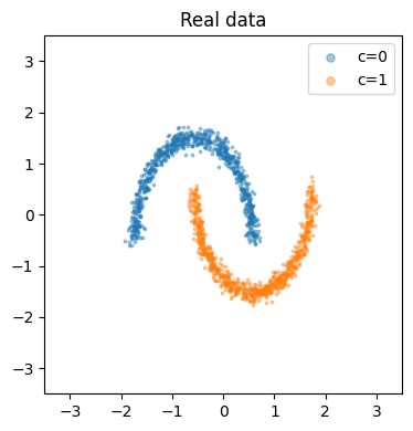

2. 构造训练路径

固定同一批起点和终点，查看不同 t t t 的插值

x t = ( 1 − t ) z + t x d a t a x_t=(1-t)z+t x_{\mathrm{data}} xt=(1−t)z+txdata

def interpolate(x_data, t, noise):
    t = t[:, None]  # [batch] -> [batch, 1]，同一个 t 用于两个坐标
    return (1 - t) * noise + t * x_data

x_demo = data[:1500]
noise_demo = torch.randn_like(x_demo)
fig, axes = plt.subplots(1, 5, figsize=(15, 3))
for ax, time in zip(axes, [0.0, 0.25, 0.5, 0.75, 1.0]):
    t = torch.full((len(x_demo),), time, device=device)
    plot_points(ax, interpolate(x_demo, t, noise_demo), f"t = {time:.2f}", conditions[:1500])
plt.tight_layout()
plt.show()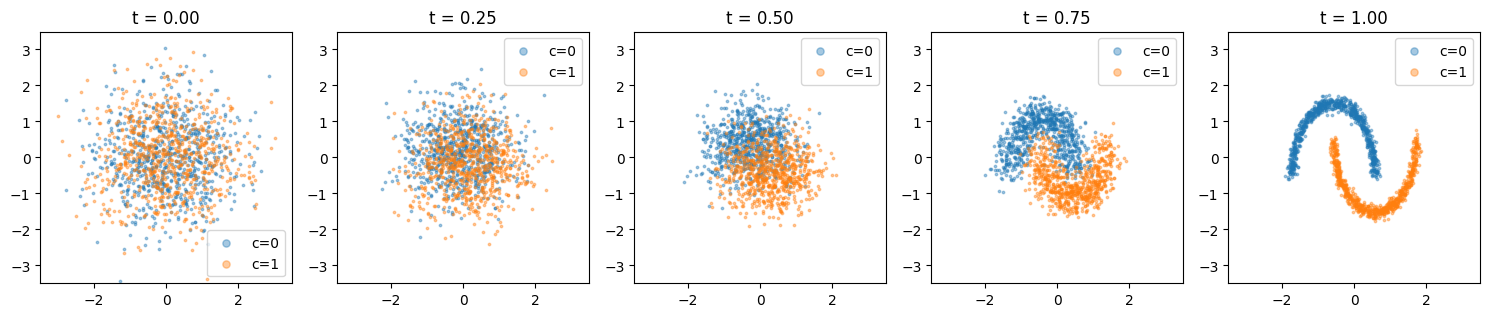

3. 条件速度预测网络

沿用原来的网络层数、宽度和时间编码，新增 8 维类别 embedding。输入维度由 18 变成 26（2 维位置 + 16 维时间编码 + 8 维条件编码）。输出仍是二维速度。时间位于 0,1，无需除以 T

class VelocityPredictor(nn.Module):
    def __init__(self, num_classes=2, condition_dim=8):
        super().__init__()
        self.register_buffer("freq", torch.arange(1, 9).float() * math.pi)
        self.condition_embedding = nn.Embedding(num_classes, condition_dim)
        self.net = nn.Sequential(
            nn.Linear(18 + condition_dim, 128), nn.SiLU(),
            nn.Linear(128, 128), nn.SiLU(),
            nn.Linear(128, 128), nn.SiLU(),
            nn.Linear(128, 2),
        )

    def forward(self, x_t, t, c):
        phase = t.float()[:, None] * self.freq[None, :]
        time_embedding = torch.cat([phase.sin(), phase.cos()], dim=1)
        condition_embedding = self.condition_embedding(c)
        return self.net(torch.cat([x_t, time_embedding, condition_embedding], dim=1))

model = VelocityPredictor().to(device)
optimizer = torch.optim.Adam(model.parameters(), lr=1e-3)

4. 条件训练

每个真实点与它的类别一起取出，噪声独立随机配对。

损失为 ∣ v θ ( x t , t , c ) − ( x d a t a − z ) ∣ 2 |v_\theta(x_t,t,c)-(x_{data}-z)|^2 ∣vθ(xt,t,c)−(xdata−z)∣2。目标速度仍是 x_data - noise，条件通过真实数据及其对应标签进入训练。不要求损失趋近零。

batch_size = 256
train_steps = 4000
loss_history = []
model.train()

for step in range(1, train_steps + 1):
    idx = torch.randint(len(data), (batch_size,), device=device)
    x_data = data[idx]
    c = conditions[idx]  # 必须与 x_data 使用同一组索引
    t = torch.rand(batch_size, device=device)
    noise = torch.randn_like(x_data)

    x_t = interpolate(x_data, t, noise)
    target_velocity = x_data - noise
    predicted_velocity = model(x_t, t, c)
    loss = (predicted_velocity - target_velocity).square().mean()

    optimizer.zero_grad()
    loss.backward()
    optimizer.step()
    loss_history.append(loss.item())

    if step % 500 == 0:
        print(f"step {step:4d} | mean loss {np.mean(loss_history[-500:]):.4f}")

plt.figure(figsize=(6, 3))
plt.plot(loss_history, alpha=0.3, label="Batch loss")
window = 100
smoothed = np.convolve(loss_history, np.ones(window) / window, mode="valid")
plt.plot(np.arange(window, len(loss_history) + 1), smoothed, label="100-step mean")
plt.xlabel("Training step")
plt.ylabel("Velocity MSE")
plt.legend()
plt.tight_layout()
plt.show()

5. 指定条件，从噪声逐步生成。

修改 condition_id=0 或 1 选择月牙。

x t + Δ t = x t + Δ t   v θ ( x t , t , c ) . x_{t+\Delta t}=x_t+\Delta t\,v_\theta(x_t,t,c). xt+Δt=xt+Δtvθ(xt,t,c).

沿用 100 步 Euler，所有步骤使用同一个网络，条件保持不变；只在初始化时抽噪声。num_steps 是数值积分步数，与训练更新次数无关。

model.eval()
num_steps = 100
condition_id = 0  # 改成 1 即可生成另一条月牙
assert condition_id in (0, 1)
snapshot_steps = sorted(set(np.linspace(0, num_steps, 5, dtype=int).tolist()))
with torch.no_grad():
    initial_noise = torch.randn(1500, 2, device=device)
    x = initial_noise.clone()
    c_gen = torch.full((len(x),), condition_id, dtype=torch.long, device=device)
    dt = 1.0 / num_steps
    snapshots = {0: x.cpu().numpy().copy()}

    for step in range(num_steps):
        t = step / num_steps
        time_batch = torch.full((len(x),), t, device=device)
        velocity = model(x, time_batch, c_gen)
        x = x + dt * velocity
        if step + 1 in snapshot_steps:
            snapshots[step + 1] = x.cpu().numpy().copy()

    generated = x.clone()

fig, axes = plt.subplots(1, len(snapshot_steps), figsize=(3 * len(snapshot_steps), 3), squeeze=False)
axes = axes.ravel()
for ax, step in zip(axes, snapshot_steps):
    plot_points(ax, snapshots[step], f"c={condition_id}, t = {step / num_steps:.2f}", c_gen)
plt.tight_layout()
plt.show()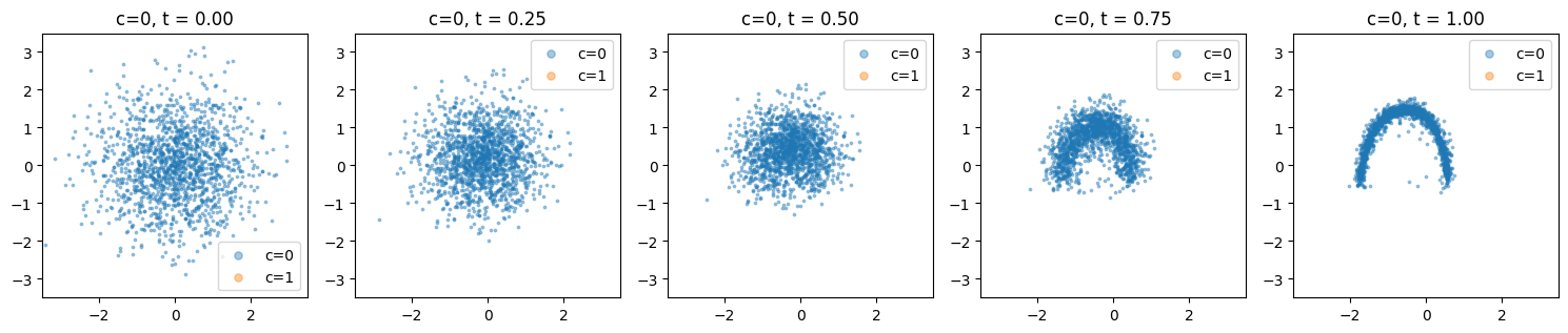

6. 相同起点和条件，一步与多步比较。

一步使用 Δ t = 1 \Delta t=1 Δt=1；直线训练不保证生成轨迹可用一步准确求解。真实数据只展示指定类别。

with torch.no_grad():
    t_zero = torch.zeros(len(initial_noise), device=device)
    one_step = initial_noise + model(initial_noise, t_zero, c_gen)

fig, axes = plt.subplots(1, 3, figsize=(12, 4))
plot_points(axes[0], data[conditions == condition_id][:1500], f"Real data: c={condition_id}")
plot_points(axes[1], one_step, "1 Euler step")
plot_points(axes[2], generated, f"{num_steps} Euler steps")
plt.tight_layout()
plt.show()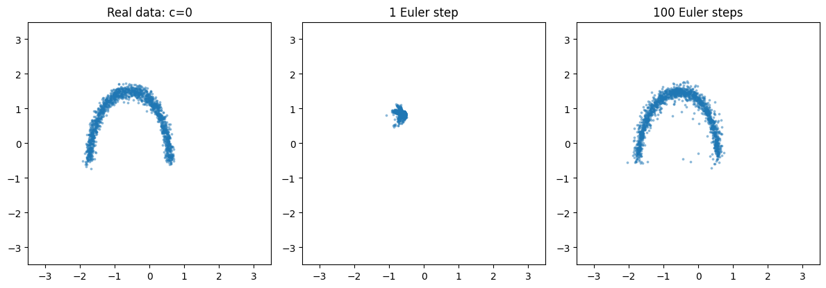

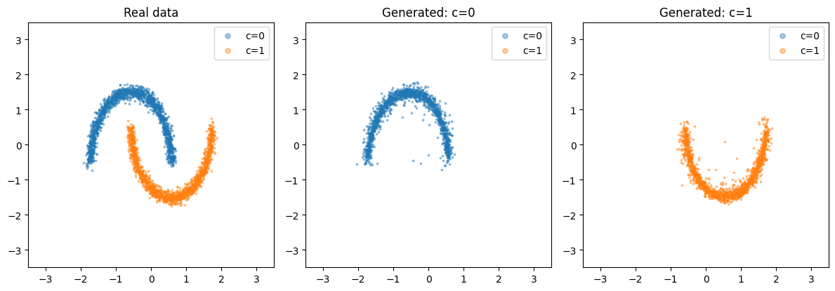
7. 相同噪声，不同条件对比

复用第 5 节的初始噪声，仅改变条件。两个条件下的生成结果应形成不同月牙；这不代表两类真实点存在已知的个体配对。

model.eval()
results = {}
with torch.no_grad():
    for label in (0, 1):
        x_cond = initial_noise.clone()
        c_cond = torch.full((len(x_cond),), label, dtype=torch.long, device=device)
        for step in range(num_steps):
            t_cond = torch.full((len(x_cond),), step / num_steps, device=device)
            x_cond = x_cond + (1.0 / num_steps) * model(x_cond, t_cond, c_cond)
        results[label] = x_cond.clone()

fig, axes = plt.subplots(1, 3, figsize=(12, 4))
plot_points(axes[0], data[:3000], "Real data", conditions[:3000])
for label in (0, 1):
    plot_points(axes[label + 1], results[label], f"Generated: c={label}",
                np.full(len(results[label]), label))
plt.tight_layout()
plt.show()