从谱图统计阈值中估计伪影（Python）

复制代码

import numpy as np
from numpy import pi as pi
import matplotlib.pyplot as plt
from src.utilities.utilstf import *
from mcsm_benchs.Benchmark import Benchmark
from src.methods.method_hard_threshold import NewMethod as ht
import librosa
from src.aps_metric.perf_metrics import aps_measure
from IPython.display import Audio
import os

plt.rc('text', usetex=True)
plt.rc('font', family='serif')

np.random.seed(0)

s,fs = librosa.load('signals/cello.wav', sr=8000)
N = 8192
xmin = 0
s = s[xmin:xmin+N]
Audio(s, rate=fs)

SNRin = 30
noise = np.random.randn(N,)
signal, scaled_noise = Benchmark.sigmerge(s,noise,SNRin,return_noise=True)
Audio(signal, rate=fs)

# Generate some example masks to show with the final figure.
Nfft = 2*1024
masks = []
thrs = np.arange(0.25,6.0,0.25)
fig, ax = plt.subplots(1,len(thrs),figsize = (4*len(thrs),5))
soutput = []


hard_thresholding =  ht().method


for i,thr in enumerate(thrs):
    
    output = hard_thresholding(signal, 
                                coeff=thr, 
                                Nfft=Nfft, 
                                dict_output=True)                          
     
    signal_output, mask2 = ( output[key] for key in 
                                    ('xr', 'mask')
                                    )
    masks.append(mask2)
    soutput.append(signal_output)
    aps_out = aps_measure(s,scaled_noise,signal_output,fs)
    ax[i].imshow(mask2,origin='lower',aspect='auto')
    
plt.show()

复制代码

# Parameters
SNRs = [0, 10, 20, 30]
reps = 30


PESQ_ht = np.zeros((len(SNRs),len(thrs),reps),)
QRF_ht = np.zeros((len(SNRs),len(thrs),5),)
APS_ht = np.zeros((len(SNRs),len(thrs),reps),)

# Load the benchmark results for the cello signal
filename = os.path.join('..','results','benchmark_cello_APS')
benchmark_aps = Benchmark.load_benchmark(filename)
df_aps = benchmark_aps.get_results_as_df() # This formats the results on a DataFrame
df_aps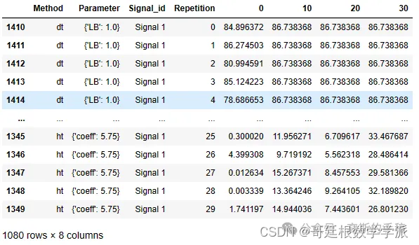

复制代码

dt_params = np.unique(df_aps['Parameter'][df_aps['Method']=='dt'])
thr_params = np.unique(df_aps['Parameter'][df_aps['Method']=='ht'])
for i,snr in enumerate(SNRs):
    for j,lb in enumerate(thr_params):
        APS_ht[i,j,:] = df_aps[snr][(df_aps['Parameter']==lb)*(df_aps['Method']=='ht')]

# Plotting APS vs. lmax from benchmark results.
fig, ax = plt.subplots(1,1, figsize=(3.8,4))


# APS vs. lambda
for q in range(len(SNRs)):
    # ax.plot(distortion,np.mean(DeltaK_PI_ht[q,:,0:8],axis=1))
    ax.plot(thrs,np.mean(APS_ht[q,:,:],axis=1),'-o',alpha=0.5,label='SNR={}'.format(SNRs[q]))


mean30 = np.mean(APS_ht[-1,:,:],axis=1)


# Insets axis with masks
# --1--
origin_inset = 1.3, 60
axins = ax.inset_axes([*origin_inset, 1.75, 30], transform=ax.transData)
axins.tick_params(axis='both', which='both', bottom=False, top=False, labelbottom=False, right=False, left=False, labelleft=False)
axins.imshow(masks[0],origin='lower',aspect='auto')
ax.plot([thrs[0],origin_inset[0]],[mean30[0],origin_inset[1]],'--k', linewidth=0.5)
ax.plot([thrs[0]],[mean30[1]],'ok', linewidth=0.5, ms=9.0,markerfacecolor='none')


# --2--
origin_inset = 1.55, 27
axins = ax.inset_axes([*origin_inset, 1.75, 30], transform=ax.transData)
axins.tick_params(axis='both', which='both', bottom=False, top=False, labelbottom=False, right=False, left=False, labelleft=False)
axins.imshow(masks[7],origin='lower',aspect='auto')
ax.plot([thrs[7],origin_inset[0]],[mean30[7],origin_inset[1]],'--k', linewidth=0.5)
ax.plot([thrs[7]],[mean30[7]],'ok', linewidth=0.5, ms=9.0, markerfacecolor='none')


# --3--
origin_inset = 4.1, 60
axins = ax.inset_axes([*origin_inset, 1.75, 30], transform=ax.transData)
axins.tick_params(axis='both', which='both', bottom=False, top=False, labelbottom=False, right=False, left=False, labelleft=False)
axins.imshow(masks[11],origin='lower',aspect='auto')
ax.plot([thrs[14],origin_inset[0]],[mean30[14],origin_inset[1]],'--k', linewidth=0.5)
ax.plot([thrs[14]],mean30[14],'ok', linewidth=0.5, ms=9.0, markerfacecolor='none')


# The spectrogram is shown in the figure for the DT method.
# origin_inset = 0.975, 0.0
# axins = ax.inset_axes([*origin_inset, 0.35, 30], transform=ax.transData)
# axins.tick_params(axis='both', which='both', bottom=False, top=False, labelbottom=False, right=False, left=False, labelleft=False)
# S, F = get_spectrogram(s,Nfft=Nfft)
# axins.imshow(np.log(np.abs(F[0:Nfft//2])+1e-6),origin='lower',aspect='auto')
# axins.imshow(S,origin='lower',aspect='auto')




ax.set_title('Hard Thresholding', fontsize=9.0)
ax.set_xlabel(r"$\lambda$", fontsize=9.0)
ax.set_ylabel(r"APS", fontsize=9.0)
# ax.legend()
ax.grid(True)


fig.savefig('figures/cello_APS_ht.pdf', dpi=900, transparent=False, bbox_inches='tight')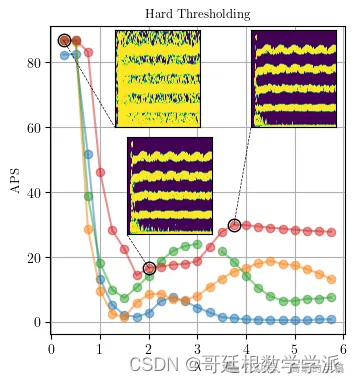

工学博士，担任《Mechanical System and Signal Processing》《中国电机工程学报》《控制与决策》等期刊审稿专家，擅长领域：现代信号处理，机器学习，深度学习，数字孪生，时间序列分析，设备缺陷检测、设备异常检测、设备智能故障诊断与健康管理PHM等。