| info | |
|---|---|
| 个人博客主页 | http://myhz0606.com/article/ncsn |
前置阅读:
DDPM: http://myhz0606.com/article/ddpm
classifier-guided:http://myhz0606.com/article/guided
classifier-free guided:http://myhz0606.com/article/classifier_free
Score based generative model:http://myhz0606.com/article/ncsn
引言
在用Stable Diffusion生成图片时,除了输入图片表述文本外(positive prompt),我们还经常会使用negative prompt作为condition来让模型避免生成negative prompt所表述的概念。查阅源码发现stable diffusion中negative prompt的实现机制是将classifier-free guided中 ϵ θ ( x t , y = ∅ , t ) \epsilon_{\theta}(x_t, y=\empty, t) ϵθ(xt,y=∅,t)替换为 ϵ θ ( x t , y ~ , t ) \epsilon_{\theta}(x_t, \tilde{y}, t) ϵθ(xt,y~,t),( y ~ \tilde{y} y~表示negative prompt)。即:
原生classifier-free guided每一个timestep的噪声估计如下:
ϵ ^ θ ( x t , y , t ) = ϵ θ ( x t , y = ∅ , t ) + s ϵ θ ( x t , y , t ) − ϵ θ ( x t , y = ∅ , t ) \begin{align} \hat{\epsilon}{\theta}(x_t, y, t)=\epsilon{\theta}(x_t, y=\empty,t) + s\\epsilon_{\\theta}(x_t, y, t) - \\epsilon_{\\theta}(x_t, y=\\empty, t) \tag{1} \end{align} ϵ^θ(xt,y,t)=ϵθ(xt,y=∅,t)+sϵθ(xt,y,t)−ϵθ(xt,y=∅,t)(1)
当有negative prompt condition时,将上式改为
ϵ ^ θ ( x t , y , t ) = ϵ θ ( x t , y ~ , t ) + s ϵ θ ( x t , y , t ) − ϵ θ ( x t , y \~ , t ) \begin{align} \hat{\epsilon}{\theta}(x_t, y, t)=\epsilon{\theta}(x_t, \tilde{y},t) + s\\epsilon_{\\theta}(x_t, y, t) - \\epsilon_{\\theta}(x_t, \\tilde{y}, t) \tag{2} \end{align} ϵ^θ(xt,y,t)=ϵθ(xt,y~,t)+sϵθ(xt,y,t)−ϵθ(xt,y\~,t)(2)
源码位置位于(diffuser版本v0.29.1): https://github.com/huggingface/diffusers/blob/main/src/diffusers/pipelines/stable_diffusion/pipeline_stable_diffusion.py#L427
那么为什么negative prompt能够work呢?
How do negative prompt take effect
为了引出相关推导,先快速回顾一下classifier-guided和classifier-free的motivation。
为了做条件生成(即从条件分布 p ( x ∣ y ) p(x|y) p(x∣y)中采样样本),我们可以根据贝叶斯公式进行如下推导:
p ( x ∣ y ) = p ( y ∣ x ) p ( x ) p ( y ) log p ( x ∣ y ) = log p ( y ∣ x ) + log p ( x ) − log p ( y ) ⇒ ∇ x log p ( x ∣ y ) = ∇ x log p ( y ∣ x ) + ∇ x log p ( x ) − ∇ x log p ( y ) ⏟ = 0 ⇒ ∇ x log p ( x ∣ y ) = ∇ x log p ( y ∣ x ) + ∇ x log p ( x ) (3) \begin{aligned} p(\mathrm{x}|y) &= \frac{p(y|\mathrm{x})p(\mathrm{x})}{p(y)} \\ \log p(\mathrm{x}|y) &= \log p(y|\mathrm{x}) + \log p(\mathrm{x}) - \log p(y) \\ \Rightarrow \nabla_{\mathrm{x}} \log p(\mathrm{x}|y) &= \nabla_{\mathrm{x}} \log p(y|\mathrm{x}) + \nabla_{\mathrm{x}} \log p(\mathrm{x}) - \underbrace{ \nabla_{\mathrm{x}} \log p(y) }{=0} \\ \Rightarrow \nabla{\mathrm{x}} \log p(\mathrm{x}|y) &= \nabla_{\mathrm{x}} \log p(y|\mathrm{x}) + \nabla_{\mathrm{x}} \log p(\mathrm{x}) \end{aligned} \tag{3} p(x∣y)logp(x∣y)⇒∇xlogp(x∣y)⇒∇xlogp(x∣y)=p(y)p(y∣x)p(x)=logp(y∣x)+logp(x)−logp(y)=∇xlogp(y∣x)+∇xlogp(x)−=0 ∇xlogp(y)=∇xlogp(y∣x)+∇xlogp(x)(3)
在classifier-guided任务中,我们已知无条件输入的score based model能够估计出 ∇ x log p ( x ) \nabla_{\mathrm{x}} \log p(\mathrm{x}) ∇xlogp(x) ,因此,为了得到 ∇ x log p ( y ∣ x ) \nabla_{\mathrm{x}} \log p(y|\mathrm{x}) ∇xlogp(y∣x) ,我们只需额外训练一个分类器来估计 ∇ x log p ( y ∣ x ) \nabla_{\mathrm{x}} \log p(y|\mathrm{x}) ∇xlogp(y∣x)即可。为了控制condition的强度,引入一个guidance scale s s s。
∇ x log p ( x ∣ y ) : = s ∇ x log p ( y ∣ x ) + ∇ x log p ( x ) (4) \nabla_{\mathrm{x}} \log p(\mathrm{x}|y) := s \nabla_{\mathrm{x}} \log p(y|\mathrm{x}) + \nabla_{\mathrm{x}} \log p(\mathrm{x}) \tag{4} ∇xlogp(x∣y):=s∇xlogp(y∣x)+∇xlogp(x)(4)
对于classifier-free任务中,通过随机drop标签,我们同时训练 ∇ x log p ( x ) \nabla_{\mathrm{x}} \log p(\mathrm{x}) ∇xlogp(x) 和 ∇ x log p ( x ∣ y ) \nabla_{\mathrm{x}} \log p(\mathrm{x}|y) ∇xlogp(x∣y) 两个score based model。虽然我们可以通过 ∇ x log p ( x ∣ y ) \nabla_{\mathrm{x}} \log p(\mathrm{x}|y) ∇xlogp(x∣y) 直接进行条件生成,但为了控制生成时条件的强度,沿用了公式(4) guidance scale的概念。并且 ∇ x log p ( y ∣ x ) = ∇ x log p ( x ∣ y ) − ∇ x log p ( x ) \nabla_{\mathrm{x}} \log p(y|\mathrm{x}) = \nabla_{\mathrm{x}} \log p(\mathrm{x}|y) - \nabla_{\mathrm{x}} \log p(\mathrm{x}) ∇xlogp(y∣x)=∇xlogp(x∣y)−∇xlogp(x) ,故有:
∇ x log p ( x ∣ y ) : = s ( ∇ x log p ( x ∣ y ) − ∇ x log p ( x ) ) + ∇ x log p ( x ) (5) \nabla_{\mathrm{x}} \log p(\mathrm{x}|y) := s (\nabla_{\mathrm{x}} \log p(\mathrm{x}|y) - \nabla_{\mathrm{x}} \log p(\mathrm{x}) ) + \nabla_{\mathrm{x}} \log p(\mathrm{x}) \tag{5} ∇xlogp(x∣y):=s(∇xlogp(x∣y)−∇xlogp(x))+∇xlogp(x)(5)
stable diffusion代码路径:https://github.com/huggingface/diffusers/blob/main/src/diffusers/pipelines/stable_diffusion/pipeline_stable_diffusion.py#L1019
当有negative prompt作为condition时,此时的condition为两项,一项是 y y y: positive prompt condition,另一项为 n o t y ~ \mathrm{not} \, \tilde{y} noty~:negative prompt condition。
只要得到 ∇ x log p ( x ∣ y , n o t y ~ ) \nabla_{\mathrm{x}} \log p(\mathrm{x}|y, \mathrm{not} \, \tilde{y}) ∇xlogp(x∣y,noty~)我们就可以参考之前的采样算法生成样本。重新直接训练一个score based model来估计 ∇ x log p ( x ∣ y , n o t y ~ ) \nabla_{\mathrm{x}} \log p(\mathrm{x}|y, \mathrm{not} \, \tilde{y}) ∇xlogp(x∣y,noty~)当然可行,但成本巨大。下面来看如何进行简化
p ( x ∣ y , n o t y ~ ) = p ( x , y , n o t y ~ ) p ( y , n o t y ~ ) = p ( y , n o t y ~ ∣ x ) p ( x ) p ( y , n o t y ~ ) = 在 x 条件下 y 与 n o t y ~ 独立 p ( y ∣ x ) p ( n o t y ~ ∣ x ) p ( x ) p ( y , n o t y ~ ) = p ( x ) p ( y , n o t y ~ ) p ( y ∣ x ) ( 1 − p ( y ~ ∣ x ) ) = p ( y ~ ∣ x ) ≠ 0 p ( x ) p ( y , n o t y ~ ) p ( y ∣ x ) ( 1 p ( y ~ ∣ x ) − 1 ) p ( y ~ ∣ x ) ∝ p ( x ) p ( y , n o t y ~ ) p ( y ∣ x ) ( 1 p ( y ~ ∣ x ) − 1 ) ∝ p ( x ) p ( y , n o t y ~ ) p ( y ∣ x ) 1 p ( y ~ ∣ x ) − p ( x ) p ( y , n o t y ~ ) p ( y ∣ x ) ∝ p ( x ) p ( y , n o t y ~ ) p ( y ∣ x ) p ( y ~ ∣ x ) ⇒ ∇ x log p ( x ∣ y , n o t y ~ ) ∝ ∇ x log p ( x ) + ∇ x log p ( y ∣ x ) − ∇ x log p ( y ~ ∣ x ) (6) \begin{aligned} p(\mathrm{x}|y, \mathrm{not}\, \tilde{y} ) & = \frac{p(\mathrm{x},y, \mathrm{not}\, \tilde{y})}{p(y, \mathrm{not}\, \tilde{y})} \\ &= \frac{p(y, \mathrm{not}\, \tilde{y}|\mathrm{x})p(\mathrm{x})}{p(y, \mathrm{not}\, \tilde{y})} \\ & \stackrel{在x条件下y与\mathrm{not} \, \tilde{y}独立}= \frac{p(y|\mathrm{x})p(\mathrm{not}\, \tilde{y}|\mathrm{x})p(\mathrm{x})}{p(y,\mathrm{not}\, \tilde{y})} \\ & = \frac{p(\mathrm{x})}{{p(y,\mathrm{not}\, \tilde{y})}} p(y|\mathrm{x}) (1 - p(\tilde{y}|\mathrm{x})) \\ & \stackrel{p(\tilde{y}|\mathrm{x}) \neq 0}= \frac{p(\mathrm{x})}{{p(y,\mathrm{not}\, \tilde{y})}} p(y|\mathrm{x}) (\frac{1}{p(\tilde{y}|\mathrm{x})} - 1) p(\tilde{y}|\mathrm{x}) \\ & \propto \frac{p(\mathrm{x})}{{p(y,\mathrm{not}\, \tilde{y})}} p(y|\mathrm{x}) (\frac{1}{p(\tilde{y}|\mathrm{x})} - 1) \\ & \propto \frac{p(\mathrm{x})}{{p(y,\mathrm{not}\, \tilde{y})}} p(y|\mathrm{x}) \frac{1}{p(\tilde{y}|\mathrm{x})} - \frac{p(\mathrm{x})}{{p(y,\mathrm{not}\, \tilde{y})}} p(y|\mathrm{x}) \\ & \propto \frac{p(\mathrm{x})}{{p(y,\mathrm{not}\, \tilde{y})}} \frac{p(y|\mathrm{x})}{p(\tilde{y}|\mathrm{x})} \\ \Rightarrow \nabla_{\mathrm{x}} \log p(\mathrm{x}|y, \mathrm{not}\, \tilde{y} ) & \propto \nabla_{\mathrm{x}} \log p(\mathrm{x}) + \nabla_{\mathrm{x}} \log p(y|\mathrm{x}) - \nabla_{\mathrm{x}} \log {p(\tilde{y}|\mathrm{x})} \end{aligned} \tag{6} p(x∣y,noty~)⇒∇xlogp(x∣y,noty~)=p(y,noty~)p(x,y,noty~)=p(y,noty~)p(y,noty~∣x)p(x)=在x条件下y与noty~独立p(y,noty~)p(y∣x)p(noty~∣x)p(x)=p(y,noty~)p(x)p(y∣x)(1−p(y~∣x))=p(y~∣x)=0p(y,noty~)p(x)p(y∣x)(p(y~∣x)1−1)p(y~∣x)∝p(y,noty~)p(x)p(y∣x)(p(y~∣x)1−1)∝p(y,noty~)p(x)p(y∣x)p(y~∣x)1−p(y,noty~)p(x)p(y∣x)∝p(y,noty~)p(x)p(y~∣x)p(y∣x)∝∇xlogp(x)+∇xlogp(y∣x)−∇xlogp(y~∣x)(6)
由于:
∇ x log p ( y ∣ x ) = ∇ x log p ( x ∣ y ) − ∇ x log p ( x ) ∇ x log p ( y ~ ∣ x ) = ∇ x log p ( x ∣ y ~ ) − ∇ x log p ( x ) (7) \begin{aligned}\nabla_{x} \log p(y|\mathrm{x}) = \nabla_{x} \log p(\mathrm{x}|y) - \nabla_{\mathrm{x}} \log p(\mathrm{x}) \\ \nabla_{\mathrm{x}} \log p(\tilde{y}|\mathrm{x}) = \nabla_{x} \log p(\mathrm{x}|\tilde{y}) - \nabla_{\mathrm{x}} \log p(\mathrm{x}) \end{aligned} \tag{7} ∇xlogp(y∣x)=∇xlogp(x∣y)−∇xlogp(x)∇xlogp(y~∣x)=∇xlogp(x∣y~)−∇xlogp(x)(7)
记 s + s^{+} s+为positive prompt condition的guidance scale, s − s^{-} s−为negative prompt的guidance scale,有
∇ x log p ( x ∣ y , n o t y ~ ) : = ∇ x log p ( x ) + s + ( ∇ x log p ( x ∣ y ) − ∇ x log p ( x ) ) − s − ( ∇ x log p ( x ∣ y ~ ) − ∇ x log p ( x ) ) (8) \nabla_{\mathrm{x}} \log p(\mathrm{x}|y, \mathrm{not}\, \tilde{y} ) := \nabla_{\mathrm{x}} \log p(\mathrm{x}) + s^{+}(\nabla_{x} \log p(\mathrm{x}|y) - \nabla_{\mathrm{x}} \log p(\mathrm{x})) - s^{-} (\nabla_{x} \log p(\mathrm{x}|\tilde{y}) - \nabla_{\mathrm{x}} \log p(\mathrm{x})) \tag{8} ∇xlogp(x∣y,noty~):=∇xlogp(x)+s+(∇xlogp(x∣y)−∇xlogp(x))−s−(∇xlogp(x∣y~)−∇xlogp(x))(8)
通过式(8)可以得出,我们只需计算 ∇ x log p ( x ) \nabla_{\mathrm{x}} \log p(\mathrm{x}) ∇xlogp(x) , ∇ x log p ( x ∣ y ) \nabla_{x} \log p(\mathrm{x}|y) ∇xlogp(x∣y), ∇ x log p ( x ∣ y ~ ) \nabla_{x} \log p(\mathrm{x}|\tilde{y}) ∇xlogp(x∣y~)三项即可估计出 ∇ x log p ( x ∣ y , n o t y ~ ) \nabla_{\mathrm{x}} \log p(\mathrm{x}|y, \mathrm{not}\, \tilde{y} ) ∇xlogp(x∣y,noty~)。
当 1 − s + + s − = 0 1 - s^{+} + s^{-} = 0 1−s++s−=0时, s − = s + − 1 s^{-} = s^{+} - 1 s−=s+−1有
∇ x log p ( x ∣ y , n o t y ~ ) = s + ∇ x log p ( x ∣ y ) − ( s + − 1 ) ∇ x log p ( x ∣ y ~ ) = ∇ x log p ( x ∣ y ~ ) + s + ( ∇ x log p ( x ∣ y ) − ∇ x log p ( x ∣ y ~ ) ) (9) \begin{aligned} \nabla_{\mathrm{x}} \log p(\mathrm{x}|y, \mathrm{not}\, \tilde{y} ) &= s^{+}\nabla_{x} \log p(\mathrm{x}|y) - (s^{+} - 1)\nabla_{x} \log p(\mathrm{x}|\tilde{y}) \\ & = \nabla_{x} \log p(\mathrm{x}|\tilde{y}) + s^{+}(\nabla_{x} \log p(\mathrm{x}|y) - \nabla_{x} \log p(\mathrm{x}|\tilde{y})) \end{aligned} \tag{9} ∇xlogp(x∣y,noty~)=s+∇xlogp(x∣y)−(s+−1)∇xlogp(x∣y~)=∇xlogp(x∣y~)+s+(∇xlogp(x∣y)−∇xlogp(x∣y~))(9)
式(9) 就是stable diffusion源码中实现形式
源码位置位于(diffuser版本v0.29.1): https://github.com/huggingface/diffusers/blob/main/src/diffusers/pipelines/stable_diffusion/pipeline_stable_diffusion.py#L427
文献3通过"Neutralization Hypothesis","Reverse Activation"解释negative prompt conditioning的工作机制,感兴趣的同学可以后续阅读。
When do negative prompt take effect
定性分析
上文我们通过理论推导证明了negative prompt conditioning的可行性。本节将从可视化的角度分析negative prompt conditioning是如何影响图片生成的。主要文献参考3
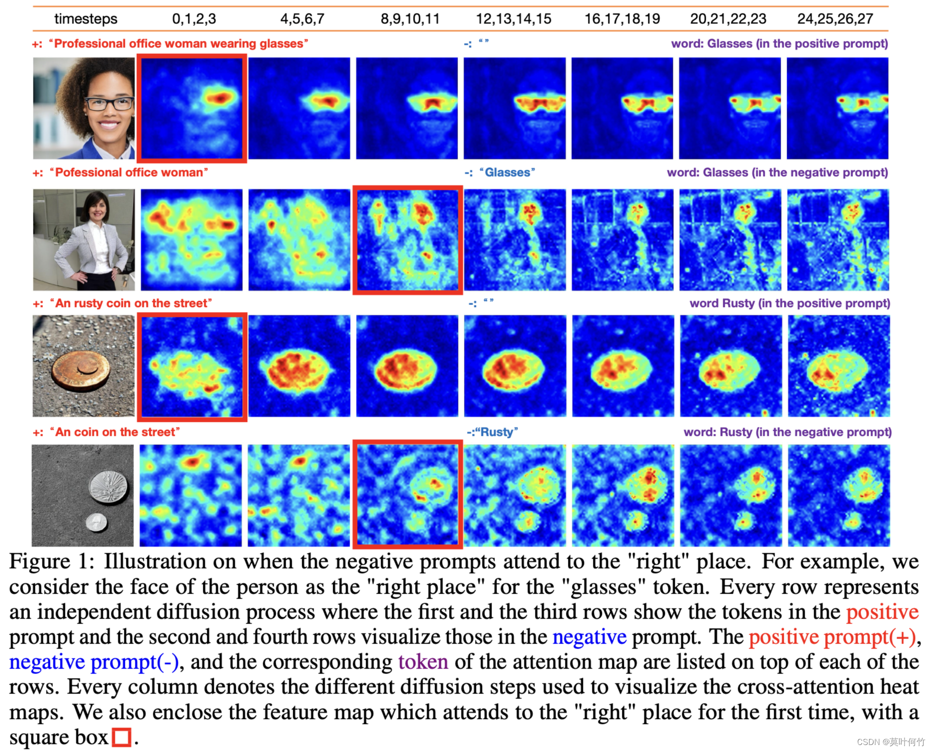
类似Prompt-to-prompt4的研究思路,我们可以绘制不同时间步token-wise attention map热力图。从图中发现,negative prompt作用存在一定延迟。positive prompt conditioning在生成的早期(t=0-3)时就关注到对应的区域,而negative prompt conditioning直到t=8-11才能正确关注到对应的区域。
定量分析
进一步的,为了定量的描述上述机制,文献3定义了 r t r_t rt为negative prompt conditioning的强度
r t = Σ k ∥ F k , p − ( i ) ( t ) ∥ F Σ k ∥ F k , p + ( r ( i ) ) ( t ) ∥ F (10) r _ { t } = \frac { \Sigma _ { k } \| F _ { k , p _ { - } ( i ) } ^ { ( t ) } \| _ { F } } { \Sigma _ { k } \| F _ { k , p _ { + } ( r ( i ) ) } ^ { ( t ) } \| _ { F } } \tag{10} rt=Σk∥Fk,p+(r(i))(t)∥FΣk∥Fk,p−(i)(t)∥F(10)
假设:Positive prompt: Pofessional office woman. Negative prompt: Glasses
p _ p_{\} p: 表示negative prompt
p + p_{+} p+: 表示positive prompt
p _ ( i ) p_{\_ }(i) p_(i):表示negative prompt第 i i i个索引处的token
p + ( r ( i ) ) p_{+}(r(i)) p+(r(i)):表示positive prompt p + p_{+} p+中与 p _ ( i ) p_{\_ }(i) p_(i)最相关的token。 p _ ( i ) p_{\_ }(i) p_(i)="Glasses", 那么 p + ( r ( i ) ) p_{+}(r(i)) p+(r(i))="woman"。
F k , p _ ( i ) t F_{k, p_{\_ (i)}}^{t} Fk,p_(i)t: 在时间步为t时,在第k层cross-attention处token p _ ( i ) p_{\_ }(i) p_(i)对应的attention map。
F k , p + ( r ( i ) ) t F_{k, p_{+}(r(i))}^{t} Fk,p+(r(i))t: 在时间步为t时,在第k层cross-attention处token p + ( r ( i ) ) p_{+}(r(i)) p+(r(i))对应的attention map。
当 r t r_t rt越小时,说明negative prompt conditioning的强度越小,反之越大。
选择了10对相应的提示对,10个不同的随机种子上进行实验,并绘制 ( r t , t ) (r_t, t) (rt,t)曲线如下:
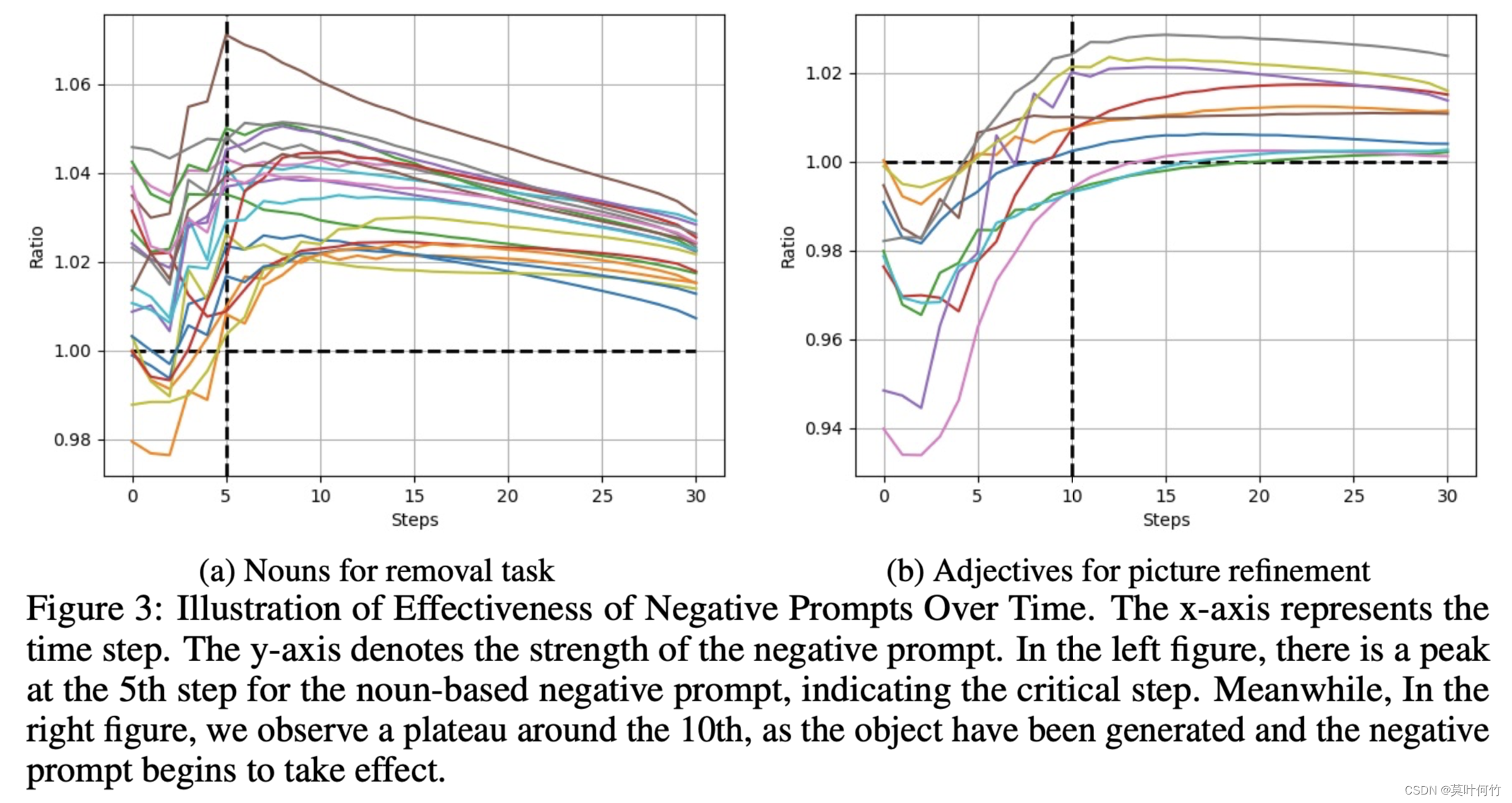
从上图不难得出:
- negative prompt conditioning的强度初始较弱,在时间步为5-10时达到峰值。
- 当negative prompt 为名词时, r t r_t rt呈先增强后降低趋势,这是由于当negative prompt作用后,会移除生成图片中的对应实体,从而让token-wise attention map的响应变弱。
- 当negative prompt 为形容词时, r t r_t rt呈先增强后稳定。
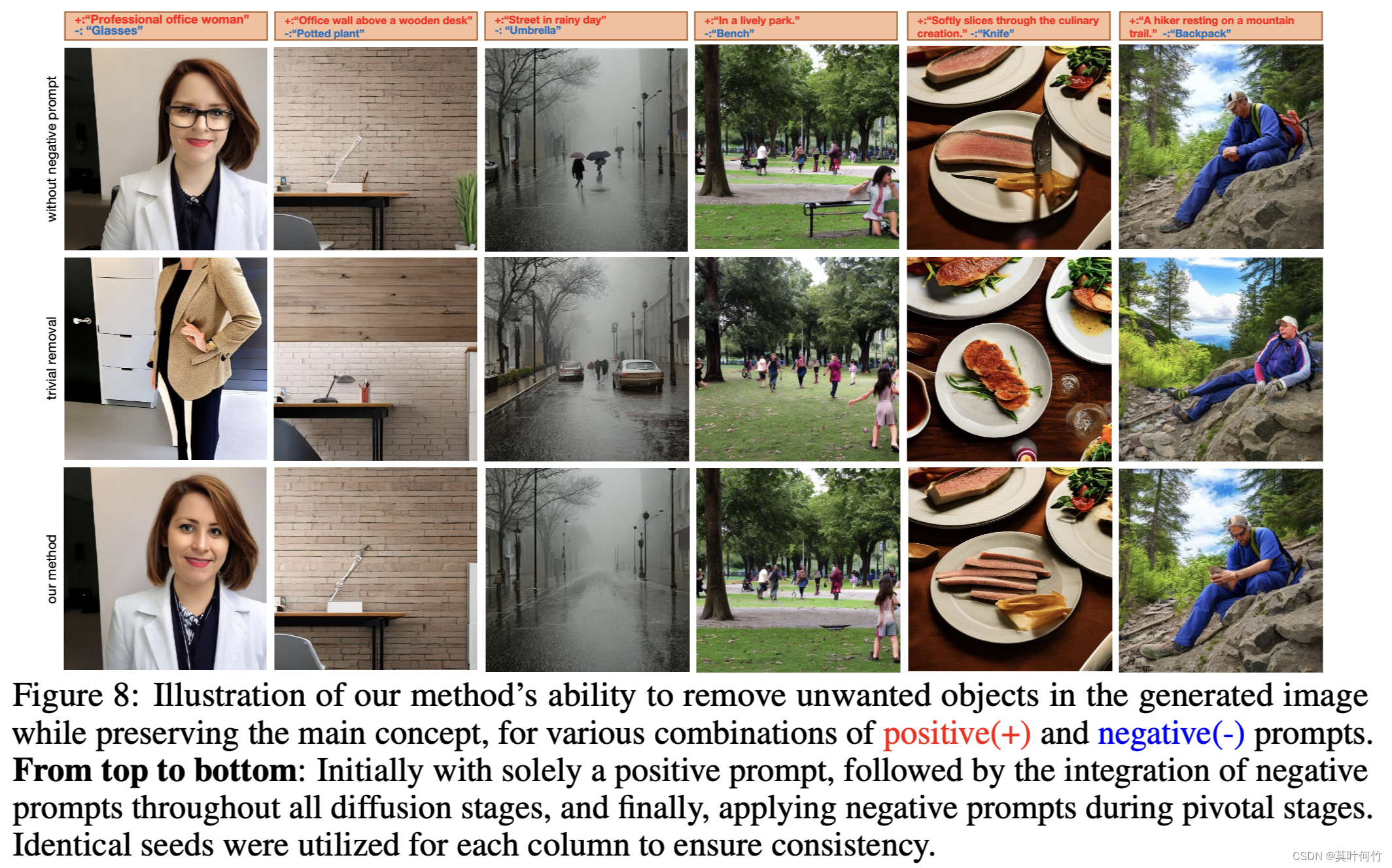
即然negative prompt conditioning存在滞后性,可以在初始阶段(t=0-5)不引入negative prompt conditioning,之后在引入,这能起到类似局部编辑的效果。
小结
本文相对系统探讨了diffusion model中negative prompt conditioning的工作机理,解释了stable diffusion关于negative prompt conditioning源码实现的合理性(式9),并给出了更一般的形式(式8)。
参考文献
1 Compositional Visual Generation with Energy Based Models
2 Compositional Visual Generation with Composable Diffusion Models
3Understanding the Impact of Negative Prompts: When and How Do They Take Effect?