案例背景

trec06c是非常经典的邮件分类的数据，还是难能可贵的中文数据集。

这个数据集从一堆txt压缩包里面提取出来整理为excel文件还真不容不易，肯定要做一下文本分类。

虽然现在文本分类基本都是深度学习了，但是传统的机器学习也能做。本案例就演示传统的贝叶斯，向量机，k近邻，这种传统模型怎么做邮件分类。

数据介绍

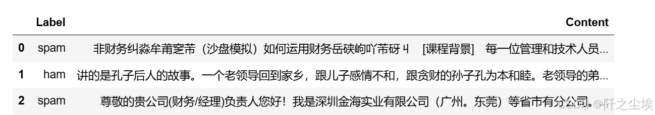
数据前3行，label是标签，spam是垃圾邮件，ham是正常邮件。content就是纯文字，中文的，还是很整洁的。

当然，需要本次案例演示数据和全部代码文件的可以参考：邮件分类

代码实现

导入需要的包、

python 复制代码

import glob,random,re,math
import pandas as pd
import numpy as np
import matplotlib.pyplot as plt
import seaborn as sns
plt.rcParams['font.sans-serif'] = ['KaiTi']  #指定默认字体 SimHei黑体
plt.rcParams['axes.unicode_minus'] = False   #解决保存图像是负号'

from collections import Counter
from wordcloud import WordCloud
from matplotlib import colors
from sklearn.feature_extraction.text import TfidfVectorizer
from sklearn.model_selection import train_test_split

读取数据

展示前3行

python 复制代码

df1=pd.read_csv('email_data.csv')
df1.head(3)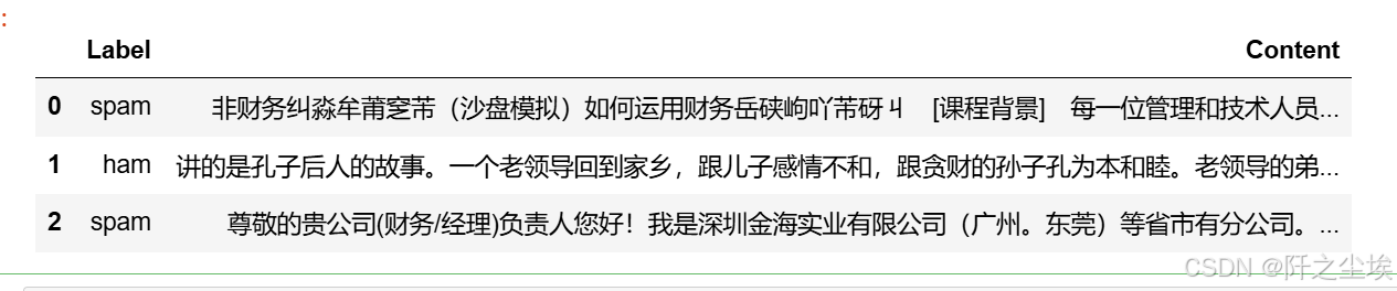

统计一下数量

python 复制代码

df1['Label'].value_counts() #统计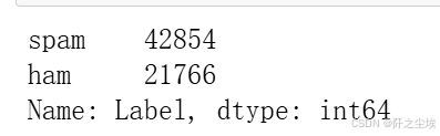

4w多的垃圾邮件，2w多的正常邮件，不平衡，我们抽取5k的正常邮件和5k的垃圾邮件合并作为数据。

数据量有点多，我正负样本都抽取5k条。

python 复制代码

# 从 DataFrame 中分别抽取 5k条垃圾邮件和 5k 条正常邮件，并合并
number=5000
df = pd.concat([
    df1[df1['Label'] == 'spam'].sample(n=number, random_state=7),  # 抽取 5k 条垃圾邮件
    df1[df1['Label'] == 'ham'].sample(n=number, random_state=7)    # 抽取 5k 条正常邮件
]).reset_index(drop=True)  # 重置索引
df['Label'].value_counts()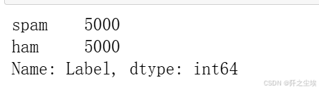

画图查看：

python 复制代码

plt.figure(figsize=(4,3),dpi=128)
sns.countplot(x=df['Label'])
#显示图像
plt.show()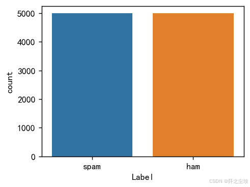

分词

中文文本都需要进行分词，需要把里面的标点符号，通用词去一下，然后变成一个个切割开的单词。

python 复制代码

import jieba     #过滤停用词，分词
stop_list  = pd.read_csv("停用词.txt",index_col=False,quoting=3,sep="\t",names=['stopword'], encoding='utf-8')
def txt_cut(juzi):         #Jieba分词函数
    lis=[w for w in jieba.lcut(juzi) if w not in stop_list.values]
    return (" ").join(lis)
df['text']=df['Content'].astype('str').apply(txt_cut)

查看前五行、

python 复制代码

df.head()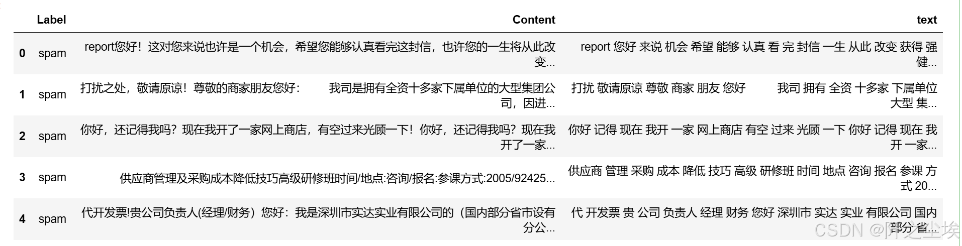

后面的文本中间都像英文的空格一样分开了。

然后，再把漏掉的标点符号，占位符，去一下

python 复制代码

df['text']=df['text'].apply(lambda x: x.replace('）','').replace('( ','').replace('－','').replace('/','').replace('（ ',''))

下面进行文本的分析

正常邮件

词频分析

这里用tf-idf的词袋方法

python 复制代码

from sklearn.feature_extraction.text import  CountVectorizer,TfidfVectorizer
from sklearn.decomposition import LatentDirichletAllocation
from sklearn.preprocessing import MinMaxScaler

将文本转为数值矩阵

python 复制代码

df_ham=df[df['Label']=='ham']  #取出正常邮件
tf_vectorizer =TfidfVectorizer()  #tf-idf词袋
#tf_vectorizer = TfidfVectorizer(ngram_range=(2,2)) #2元词袋
X = tf_vectorizer.fit_transform(df_ham['text'])
print(X.shape)

feature_names = tf_vectorizer.get_feature_names_out()
tfidf_values = X.toarray()
print(feature_names.shape,tfidf_values.shape)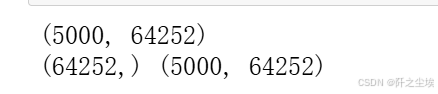

查看对应的词汇名称，tf-idf的值，权重等

python 复制代码

# 从转换器中提取词汇和对应的 TF-IDF 值
data1 = {'word': tf_vectorizer.get_feature_names_out(),
        'frequency':np.count_nonzero(X.toarray(), axis=0),
        'weight': X.mean(axis=0).A.flatten(),}
df1 = pd.DataFrame(data1).sort_values(by="frequency" ,ascending=False,ignore_index=True) 
df1.head()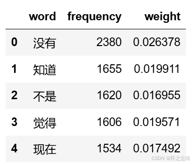

可以储存一下

python 复制代码

#储存
df1.to_excel('正常邮件词频.xlsx', index=False)

查看评率最高前20的词汇

python 复制代码

#前20个频率最高的词汇
df2=pd.DataFrame(data1).sort_values(by="frequency" ,ascending=False,ignore_index=True) 
plt.figure(figsize=(7,3),dpi=256)
sns.barplot(x=df2['word'][:20],y=df2['frequency'][:20])
plt.xticks(rotation=70,fontsize=9) 
plt.ylabel('频率')
plt.xlabel('')
#plt.title('前20个频率最高的词汇')
plt.show()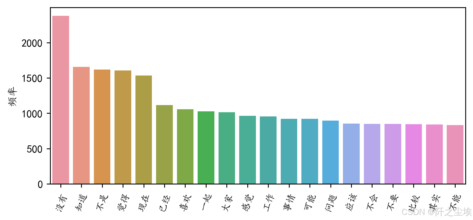

词云图

画出对应的词云图

python 复制代码

#定义随机生成颜色函数
def randomcolor():
    colorArr = ['1','2','3','4','5','6','7','8','9','A','B','C','D','E','F']
    color ="#"+''.join([random.choice(colorArr) for i in range(6)])
    return color

#from imageio import imread    #形状设置
#mask = imread('爱心.png')  
all_titles = ' '.join(df_ham['text'])
# Word segmentation
seg_list = jieba.cut(all_titles, cut_all=False)
seg_text = ' '.join(seg_list)     
#对分词文本做高频词统计
word_counts = Counter(seg_text.split())
word_counts_updated=word_counts.most_common()
#过滤标点符号
non_chinese_pattern = re.compile(r'[^\u4e00-\u9fa5]')
# 过滤掉非中文字符的词汇
filtered_word_counts_regex = [item for item in word_counts_updated if not non_chinese_pattern.match(item[0])]
filtered_word_counts_regex[:5]

python 复制代码

# Generate word cloud
wordcloud = WordCloud(font_path='simhei.ttf', background_color='white', 
                      max_words=80,        # Limits the number of words to 100
                      max_font_size=50)   #.generate(seg_text)    #文本可以直接生成，但是不好看
wordcloud = wordcloud.generate_from_frequencies(dict(filtered_word_counts_regex))
# Display the word cloud
plt.figure(figsize=(8, 5),dpi=256)
plt.imshow(wordcloud, interpolation='bilinear')
plt.axis('off')
plt.show()

上面都是正常邮件的词汇分析，下面就是垃圾邮件的分析

垃圾邮件

词频分析

转为tf-idf的词矩阵

python 复制代码

df_spam=df[df['Label']=='spam']
tf_vectorizer =TfidfVectorizer()
#tf_vectorizer = TfidfVectorizer(ngram_range=(2,2)) #2元词袋
X = tf_vectorizer.fit_transform(df_spam['text'])
#print(tf_vectorizer.get_feature_names_out())
print(X.shape)

feature_names = tf_vectorizer.get_feature_names_out()
tfidf_values = X.toarray()
print(feature_names.shape,tfidf_values.shape)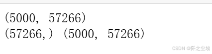

从转换器中提取词汇和对应的 TF-IDF 值

python 复制代码

data1 = {'word': tf_vectorizer.get_feature_names_out(),
        'frequency':np.count_nonzero(X.toarray(), axis=0),
        'weight': X.mean(axis=0).A.flatten(),}
df1 = pd.DataFrame(data1).sort_values(by="frequency" ,ascending=False,ignore_index=True) 
df1.head()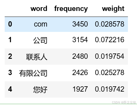

储存一下，可以看到com较多，说明垃圾邮件里面的很多网址链接

也可以储存一下

python 复制代码

#储存
df1.to_excel('垃圾邮件词频.xlsx', index=False)

前20个词汇

python 复制代码

#前20个频率最高的词汇
df2=pd.DataFrame(data1).sort_values(by="frequency" ,ascending=False,ignore_index=True) 
plt.figure(figsize=(7,3),dpi=256)
sns.barplot(x=df2['word'][:20],y=df2['frequency'][:20])
plt.xticks(rotation=70,fontsize=9) 
plt.ylabel('频率')
plt.xlabel('')
#plt.title('前20个频率最高的词汇')
plt.show()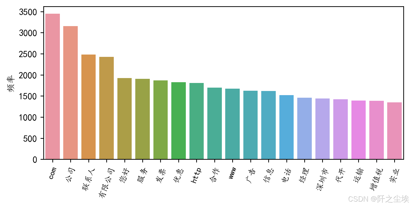

词云图

python 复制代码

#from imageio import imread    #形状设置
#mask = imread('爱心.png')  
all_titles = ' '.join(df_spam['text'])
# Word segmentation
seg_list = jieba.cut(all_titles, cut_all=False)
seg_text = ' '.join(seg_list)     
#对分词文本做高频词统计
word_counts = Counter(seg_text.split())
word_counts_updated=word_counts.most_common()
#过滤标点符号
non_chinese_pattern = re.compile(r'[^\u4e00-\u9fa5]')
# 过滤掉非中文字符的词汇
filtered_word_counts_regex = [item for item in word_counts_updated if not non_chinese_pattern.match(item[0])]
filtered_word_counts_regex[:5]

python 复制代码

# Generate word cloud
wordcloud = WordCloud(font_path='simhei.ttf', background_color='white', 
                      max_words=80,        # Limits the number of words to 100
                      max_font_size=50)   #.generate(seg_text)    #文本可以直接生成，但是不好看
wordcloud = wordcloud.generate_from_frequencies(dict(filtered_word_counts_regex))
# Display the word cloud
plt.figure(figsize=(8, 5),dpi=256)
plt.imshow(wordcloud, interpolation='bilinear')
plt.axis('off')
plt.show()

机器学习

#准备X和y，还是一样的tf-idf的词表矩阵，这里限制一下矩阵的维度为5000，免得数据维度太大了训练时间很长。

python 复制代码

#取出X和y
X = df['text']
y = df['Label']
#创建一个TfidfVectorizer的实例
vectorizer = TfidfVectorizer(max_features=5000,max_df=0.1,min_df=3)
#使用Tfidf将文本转化为向量
X = vectorizer.fit_transform(X)
#看看特征形状
X.shape

查看词汇频率

python 复制代码

data1 = {'word': vectorizer.get_feature_names_out(),
        'tfidf': X.toarray().sum(axis=0).tolist()}
df1 = pd.DataFrame(data1).sort_values(by="tfidf" ,ascending=False,ignore_index=True) 
df1.head(10)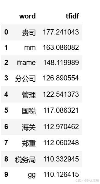

划分训练集和测试集

y映射一下，变成数值型

python 复制代码

y1=y.map({'spam':1,'ham':0})
X_train, X_test, y_train, y_test =train_test_split(X,y,test_size=0.2,stratify=y,random_state = 0)
#可以检查一下划分后数据形状
X_train.shape,X_test.shape, y_train.shape, y_test.shape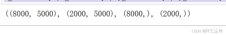

模型对比

python 复制代码

#采用三种模型，对比测试集精度
from sklearn.naive_bayes import MultinomialNB
from sklearn.neighbors import KNeighborsClassifier
from sklearn.svm import SVC

实例化模型

python 复制代码

#朴素贝叶斯
model1 = MultinomialNB()
#K近邻
model2 = KNeighborsClassifier(n_neighbors=100)
#支持向量机
model3 = SVC(kernel="rbf", random_state=77, probability=True)

model_list=[model1,model2,model3]
model_name=['朴素贝叶斯','K近邻','支持向量机']

自定义一下训练和评价函数

python 复制代码

from sklearn.metrics import confusion_matrix, roc_curve, auc
from sklearn.metrics import ConfusionMatrixDisplay

def evaluate_model(model, X_train, X_test, y_train, y_test, model_name):
    # 训练模型
    model.fit(X_train, y_train)
    
    # 计算准确率
    accuracy = model.score(X_test, y_test)
    print(f'{model_name}方法在测试集的准确率为{round(accuracy, 3)}')
    
    # 计算混淆矩阵
    cm = confusion_matrix(y_test, model.predict(X_test))
    print(f'混淆矩阵：\n{cm}')
    
    # 绘制混淆矩阵热力图
    disp = ConfusionMatrixDisplay(confusion_matrix=cm, display_labels=['spam', 'ham'])
    disp.plot(cmap=plt.cm.Blues)
    plt.title(f'Confusion Matrix - {model_name}')
    plt.show()
    
    # 计算 ROC 曲线
    fpr, tpr, thresholds = roc_curve(y_test, model.predict_proba(X_test)[:, 1], pos_label='spam')
    roc_auc = auc(fpr, tpr)
    
    # 绘制 ROC 曲线
    plt.plot(fpr, tpr, label=f'{model_name} (AUC = {roc_auc:.6f})')
    plt.xlabel('False Positive Rate')
    plt.ylabel('True Positive Rate')
    plt.title('ROC Curve')
    plt.legend()
    plt.show()

    return accuracy

对三个模型都进行一下训练

python 复制代码

accuracys=[]
for model, name in zip(model_list, model_name):
    accuracy=evaluate_model(model, X_train, X_test, y_train, y_test, name)
    accuracys.append(accuracy)

这个函数会画出很多图，混淆矩阵，ROC的图，评价指标等。

查看三个模型的准确率

python 复制代码

accuracys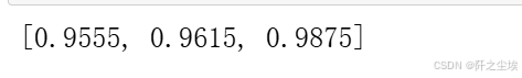

准确率进行可视化

python 复制代码

plt.figure(figsize=(7,3),dpi=128)
sns.barplot(y=model_name,x=accuracys,orient="h")
plt.xlabel('模型准确率')
plt.ylabel('模型名称')
plt.xticks(fontsize=10,rotation=45)
plt.title("不同模型文本分类准确率对比")
plt.show()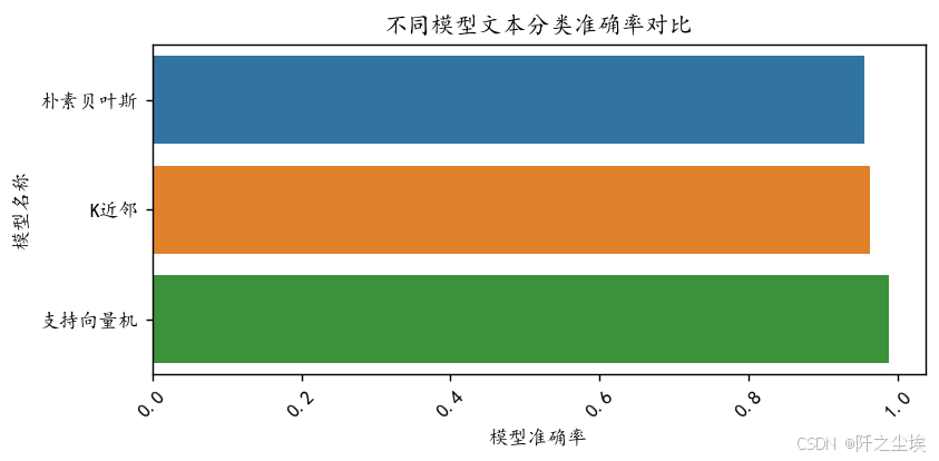

支持向量机准确率最高！

ROC对比

python 复制代码

plt.figure(figsize=(8, 6),dpi=128)

# 遍历每个模型，绘制其 ROC 曲线
for model, name in zip(model_list, model_name):
    model.fit(X_train, y_train)  # 训练模型
    fpr, tpr, _ = roc_curve(y_test, model.predict_proba(X_test)[:, 1], pos_label='spam')  # 计算 ROC 曲线的参数
    roc_auc = auc(fpr, tpr)  # 计算 AUC
    plt.plot(fpr, tpr, label=f'{name} (AUC = {roc_auc:.6f})')  # 绘制 ROC 曲线

# 绘制对角线
plt.plot([0, 1], [0, 1], linestyle='--', color='grey', label='Random')
# 设置图形属性
plt.xlabel('False Positive Rate')
plt.ylabel('True Positive Rate')
plt.title('ROC Curve')
plt.legend()
plt.show()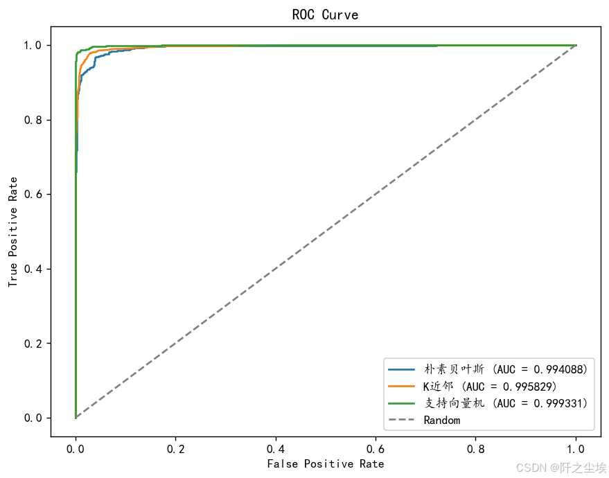

支持向量机的auc最高。

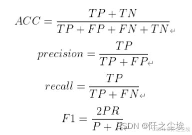
四个评价指标

模型再实例化一下，我们计算分类问题常用的四个评价指标，准确率，精准度，召回率，F1值

python 复制代码

from sklearn.metrics import confusion_matrix
from sklearn.metrics import classification_report
from sklearn.metrics import cohen_kappa_score
#朴素贝叶斯
model1 = MultinomialNB()
#K近邻
model2 = KNeighborsClassifier(n_neighbors=100)
#支持向量机
model3 = SVC(kernel="rbf", random_state=77, probability=True)

model_list=[model1,model2,model3]
#model_name=['朴素贝叶斯','K近邻','支持向量机']

自定义评价指标

python 复制代码

def evaluation(y_test, y_predict):
    accuracy=classification_report(y_test, y_predict,output_dict=True)['accuracy']
    s=classification_report(y_test, y_predict,output_dict=True)['weighted avg']
    precision=s['precision']
    recall=s['recall']
    f1_score=s['f1-score']
    #kappa=cohen_kappa_score(y_test, y_predict)
    return accuracy,precision,recall,f1_score #, kappa
def evaluation2(lis):
    array=np.array(lis)
    return array.mean() , array.std()

循环，遍历，预测，计算评价指标

python 复制代码

df_eval=pd.DataFrame(columns=['Accuracy','Precision','Recall','F1_score'])
for i in range(3):
    model_C=model_list[i]
    name=model_name[i]
    model_C.fit(X_train, y_train)
    pred=model_C.predict(X_test)
    s=classification_report(y_test, pred)
    s=evaluation(y_test,pred)
    df_eval.loc[name,:]=list(s)

查看

python 复制代码

df_eval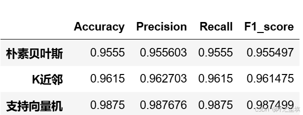

可视化

python 复制代码

bar_width = 0.4
colors = ['c', 'g', 'tomato', 'b', 'm', 'y', 'lime', 'k', 'orange', 'pink', 'grey', 'tan']
fig, axes = plt.subplots(2, 2, figsize=(7, 6), dpi=128)

for i, col in enumerate(df_eval.columns):
    ax = axes[i//2, i%2]  # 这将为每个子图指定一个轴
    df_col = df_eval[col]
    m = np.arange(len(df_col))
    bars = ax.bar(x=m, height=df_col.to_numpy(), width=bar_width, color=colors)

    # 在柱状图上方显示数值
    for bar in bars:
        yval = bar.get_height()
        ax.text(bar.get_x() + bar.get_width()/2, yval, round(yval, 4), ha='center', va='bottom', fontsize=8)

    # 设置x轴
    names = df_col.index
    ax.set_xticks(range(len(df_col)))
    ax.set_xticklabels(names, fontsize=10, rotation=40)

    # 设置y轴
    ax.set_ylim([0.94, df_col.max() + 0.02]) 
    ax.set_ylabel(col, fontsize=14)

plt.tight_layout()
# plt.savefig('柱状图.jpg', dpi=512)  # 如果需要保存图片取消注释这行
plt.show()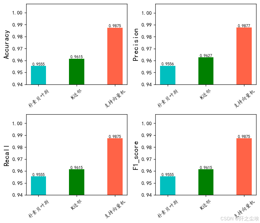

很明显支持向量机效果最好

交叉验证

自定义交叉验证评价指标和函数

python 复制代码

def evaluation(y_test, y_predict):
    accuracy=classification_report(y_test, y_predict,output_dict=True)['accuracy']
    s=classification_report(y_test, y_predict,output_dict=True)['weighted avg']
    precision=s['precision']
    recall=s['recall']
    f1_score=s['f1-score']
    #kappa=cohen_kappa_score(y_test, y_predict)
    return accuracy,precision,recall,f1_score #, kappa
def evaluation2(lis):
    array=np.array(lis)
    return array.mean() , array.std()

python 复制代码

from sklearn.model_selection import KFold
def cross_val(model=None,X=None,Y=None,K=5,repeated=1,show_confusion_matrix=True):
    df_mean=pd.DataFrame(columns=['Accuracy','Precision','Recall','F1_score']) 
    df_std=pd.DataFrame(columns=['Accuracy','Precision','Recall','F1_score'])
    for n in range(repeated):
        print(f'正在进行第{n+1}次重复K折.....随机数种子为{n}\n')
        kf = KFold(n_splits=K, shuffle=True, random_state=n)
        Accuracy=[]
        Precision=[]
        Recall=[]
        F1_score=[]
        print(f"    开始本次在{K}折数据上的交叉验证.......\n")
        i=1
        for train_index, test_index in kf.split(X):
            print(f'        正在进行第{i}折的计算')
            X_train=X[train_index]
            y_train=np.array(y)[train_index]
            X_test=X[test_index]
            y_test=np.array(y)[test_index]
            model.fit(X_train,y_train)
            pred=model.predict(X_test)
            score=list(evaluation(y_test,pred))
            Accuracy.append(score[0])
            Precision.append(score[1])
            Recall.append(score[2])
            F1_score.append(score[3])
            
            if show_confusion_matrix:
                #数据透视表，混淆矩阵
                print("混淆矩阵：")
                table = pd.crosstab(y_test, pred, rownames=['Actual'], colnames=['Predicted'])
                #print(table)
                plt.figure(figsize=(4,3))
                sns.heatmap(table,cmap='Blues',fmt='.20g', annot=True)
                plt.tight_layout()
                plt.show()
                #计算混淆矩阵的各项指标
                print('混淆矩阵的各项指标为：')
                print(classification_report(y_test, pred))
                
            print(f'        第{i}折的准确率为：{round(score[0],4)}，Precision为{round(score[1],4)}，Recall为{round(score[2],4)}，F1_score为{round(score[3],4)}')
            i+=1
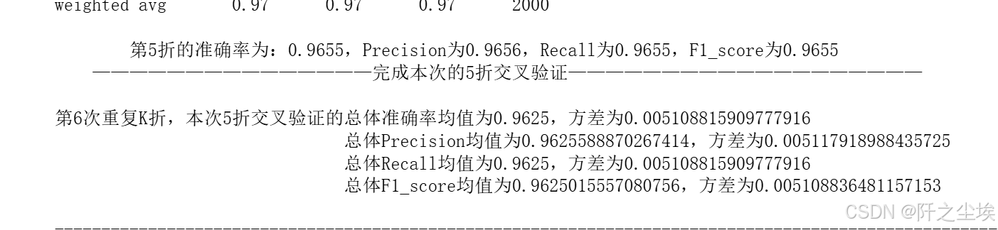
        print(f'    ---------------------------------------------完成本次的{K}折交叉验证---------------------------------------------------------\n')
        Accuracy_mean,Accuracy_std=evaluation2(Accuracy)
        Precision_mean,Precision_std=evaluation2(Precision)
        Recall_mean,Recall_std=evaluation2(Recall)
        F1_score_mean,F1_score_std=evaluation2(F1_score)
        print(f'第{n+1}次重复K折，本次{K}折交叉验证的总体准确率均值为{Accuracy_mean}，方差为{Accuracy_std}')
        print(f'                               总体Precision均值为{Precision_mean}，方差为{Precision_std}')
        print(f'                               总体Recall均值为{Recall_mean}，方差为{Recall_std}')
        print(f'                               总体F1_score均值为{F1_score_mean}，方差为{F1_score_std}')
        print("\n====================================================================================================================\n")
        df1=pd.DataFrame(dict(zip(['Accuracy','Precision','Recall','F1_score'],[Accuracy_mean,Precision_mean,Recall_mean,F1_score_mean])),index=[n])
        df_mean=pd.concat([df_mean,df1])
        df2=pd.DataFrame(dict(zip(['Accuracy','Precision','Recall','F1_score'],[Accuracy_std,Precision_std,Recall_std,F1_score_std])),index=[n])
        df_std=pd.concat([df_std,df2])
    return df_mean,df_std

实例化三个模型

python 复制代码

model1 = MultinomialNB()
#K近邻
model2 = KNeighborsClassifier(n_neighbors=100)
#支持向量机
model3 = SVC(kernel="rbf", random_state=77, probability=True)

贝叶斯：

python 复制代码

model =MultinomialNB()
nb_crosseval,nb_crosseval2=cross_val(model=model,X=X,Y=y,K=5,repeated=6)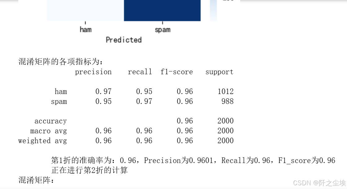

结果都打印出来的。

朴素贝叶斯的评价指标

python 复制代码

nb_crosseval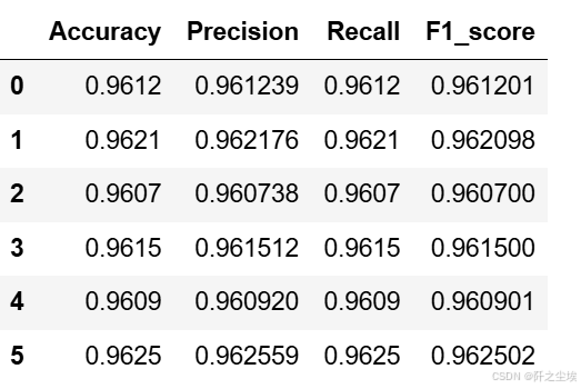

K近邻

python 复制代码

model =KNeighborsClassifier(n_neighbors=100)
knn_crosseval,knn_crosseval2=cross_val(model=model,X=X,Y=y,K=5,repeated=6,show_confusion_matrix=False)

不放过程了，直接上结果

python 复制代码

knn_crosseval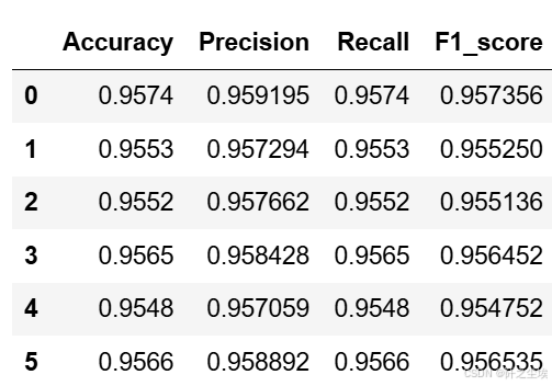

支持向量机

python 复制代码

model = SVC(kernel="rbf", random_state=77, probability=True)
svc_crosseval,svc_crosseval2=cross_val(model=model,X=X,Y=y,K=5,repeated=6,show_confusion_matrix=False)

评价指标

python 复制代码

svc_crosseval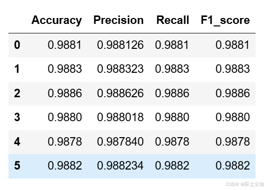

均值的可视化

python 复制代码

plt.subplots(1,4,figsize=(16,3),dpi=128)
for i,col in enumerate(nb_crosseval.columns):
    n=int(str('14')+str(i+1))
    plt.subplot(n)
    plt.plot(nb_crosseval[col], 'k', label='NB')
    plt.plot(knn_crosseval[col], 'b-.', label='KNN')
    plt.plot(svc_crosseval[col], 'r-^', label='SVC')
    plt.title(f'不同模型的{col}对比')
    plt.xlabel('重复交叉验证次数')
    plt.ylabel(col,fontsize=16)
    plt.legend()
plt.tight_layout()
plt.show()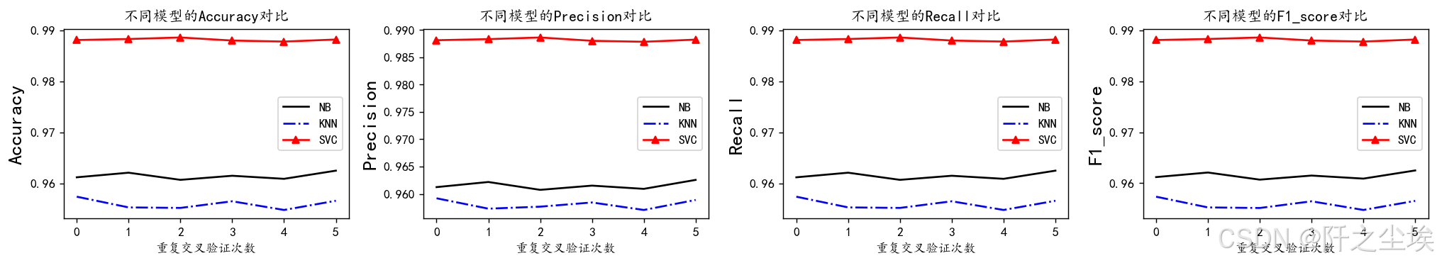

方差的可视化

python 复制代码

plt.subplots(1,4,figsize=(16,3),dpi=128)
for i,col in enumerate(nb_crosseval2.columns):
    n=int(str('14')+str(i+1))
    plt.subplot(n)
    plt.plot(nb_crosseval2[col], 'k', label='NB')
    plt.plot(knn_crosseval2[col], 'b-.', label='KNN')
    plt.plot(svc_crosseval2[col], 'r-^', label='SVC')
    plt.title(f'不同模型的{col}方差对比')
    plt.xlabel('重复交叉验证次数')
    plt.ylabel(col,fontsize=16)
    plt.legend()
plt.tight_layout()
plt.show()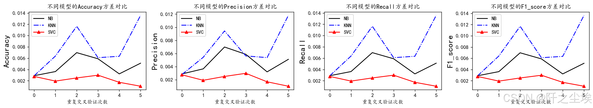

结论：

我们将进行三种机器学习模型的性能分析：朴素贝叶斯（Naive Bayes）、k近邻（k-Nearest Neighbors）和支持向量机（Support Vector Machine）。

1. 朴素贝叶斯模型分析：

朴素贝叶斯模型在数据集上表现出了相对较高的性能。具体来说，它在准确率（Accuracy）、精确率（Precision）、召回率（Recall）和F1分数（F1-score）方面均取得了稳定的表现，分别达到了约96%的水平。这表明朴素贝叶斯模型在数据分类方面具有较高的效果，并且不易受到数据波动的影响。

2. k近邻模型分析：

与朴素贝叶斯相比，k近邻模型在性能上稍显不及。尽管其在准确率和F1分数方面表现相当，但在精确率和召回率方面略有下降，分别在95%左右。这可能表明k近邻模型在处理数据集中的某些特征时存在一定的困难，导致了一些分类错误。

3. 支持向量机模型分析：

支持向量机（SVM）模型在这份数据集上展现了最佳的性能。其在所有评估指标上均表现出了接近98%的高水平，包括准确率、精确率、召回率和F1分数。这表明支持向量机模型在数据分类任务中具有较强的鲁棒性和泛化能力，能够有效地捕捉数据之间的复杂关系，并进行准确的分类。

综上所述，支持向量机模型在这份数据集上表现最佳，其稳定性和高性能使其成为首选模型。朴素贝叶斯模型在某些情况下也是一个可行的选择，而k近邻模型可能需要进一步优化以提高其性能。

支持向量机的准确率最高，模型波动的方差小，效果最好，下面对它进行超参数搜索。

超参数搜索

python 复制代码

#利用K折交叉验证搜索最优超参数
from sklearn.model_selection import KFold, StratifiedKFold
from sklearn.model_selection import GridSearchCV,RandomizedSearchCV

参数范围

python 复制代码

param_grid = {
    'C': [0.1, 1, 10],
    'gamma': [ 0.01, 0.1, 1, 10]}

model = GridSearchCV(estimator=SVC(kernel="rbf"), param_grid=param_grid, cv=3)
model.fit(X_train, y_train)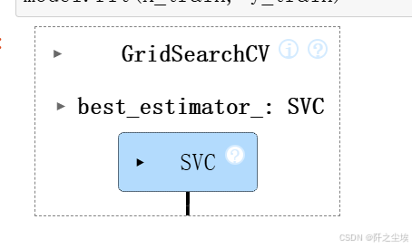

参数

python 复制代码

model.best_params_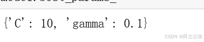

评估

python 复制代码

model = model.best_estimator_
pred=model.predict(X_test)
evaluation(y_test,pred)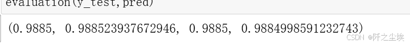

对这个区间再度细化搜索

python 复制代码

param_grid = {
    'C': [6,7,8,9,10,11,12,13,14],
    'gamma': [ 0.08,0.09,0.1,0.15,0.2,0.3]}

model = GridSearchCV(estimator=SVC(kernel="rbf"), param_grid=param_grid, cv=3)
model.fit(X_train, y_train)

python 复制代码

model.best_params_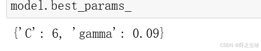

python 复制代码

model = model.best_estimator_
pred=model.predict(X_test)
evaluation(y_test,pred)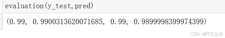

能达到99%准确率了。

画图：

python 复制代码

import itertools
def plot_confusion_matrix(cm, classes,title='Confusion matrix',cmap=plt.cm.Blues):
    plt.imshow(cm, interpolation='nearest', cmap=cmap)
    plt.title(title)
    plt.colorbar()
    tick_marks = np.arange(len(classes))
    plt.xticks(tick_marks, classes, rotation=0)
    plt.yticks(tick_marks, classes)
 
    thresh = cm.max() / 2.
    for i, j in itertools.product(range(cm.shape[0]), range(cm.shape[1])):
        plt.text(j, i, cm[i, j],
                 horizontalalignment="center",
                 color="white" if cm[i, j] > thresh else "black")
    plt.tight_layout()
    plt.ylabel('True label')
    plt.xlabel('Predicted label')

最好的模型：

python 复制代码

import time 
svc=SVC(kernel="rbf",C=6  , gamma=0.09)
startTime = time.time()
svc.fit(X_train, y_train)
print('svc分类器训练用时%.2f秒' %(time.time()-startTime))
pred=svc.predict(X_test)
print(f"准确率，精确度，召回率，F1值：{np.round(evaluation(y_test,pred),6)}")
plot_confusion_matrix(confusion_matrix(y_test,pred),[0,1])
plt.show()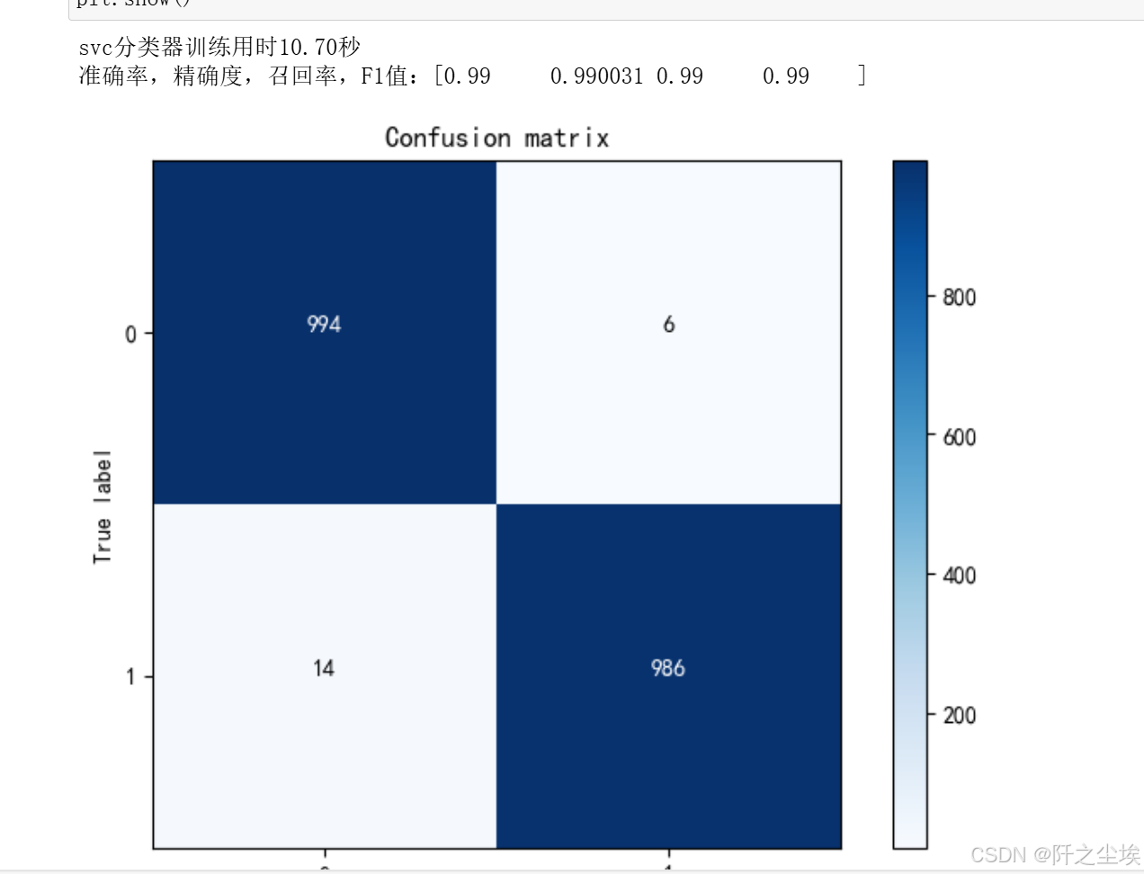

模型保存

python 复制代码

import joblib
# 模型已经选取了最佳估计器，存储在变量 model 中
# 保存模型到文件
joblib.dump(model, 'best_model.pkl')

加载模型，然后预测

python 复制代码

# 加载模型
loaded_model = joblib.load('best_model.pkl')
# 使用加载的模型进行预测
loaded_model.predict(X_test)
evaluation(y_test, pred)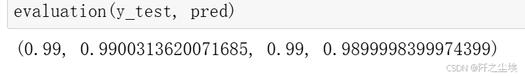

基本是99%的准确率，还是很好用的。

创作不易，看官觉得写得还不错的话点个关注和赞吧，本人会持续更新python数据分析领域的代码文章~(需要定制类似的代码可私信)

Python数据分析案例49——基于机器学习的垃圾邮件分类系统构建(朴素贝叶斯，支持向量机)

案例背景

数据介绍

代码实现

读取数据

分词

正常邮件

词频分析

词云图

垃圾邮件

词频分析

从转换器中提取词汇和对应的 TF-IDF 值

词云图

机器学习

划分训练集和测试集

模型对比

四个评价指标

交叉验证

1. 朴素贝叶斯模型分析：

2. k近邻模型分析：

3. 支持向量机模型分析：

超参数搜索

模型保存