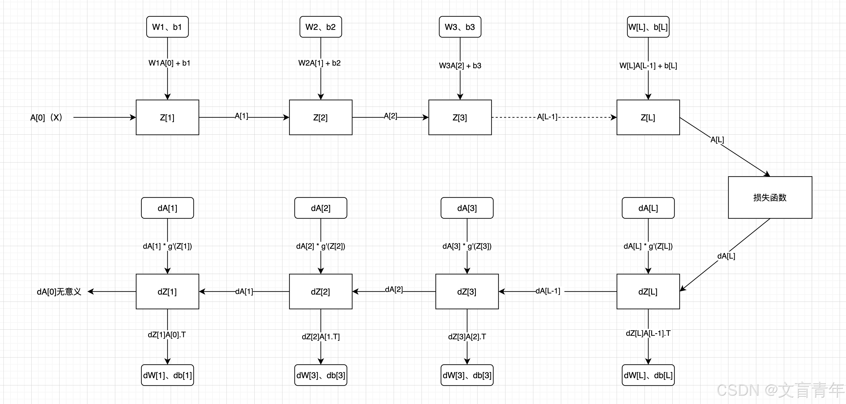
维度说明:
AL、ZL:(本层神经元个数、样本数)
WL:(本层神经元个数、上层神经元个数)
bL:(本层神经元个数、1)
dZL:dAL * g'A(ZL)dZL:(本层神经元个数、样本数)
dw = dL/dz * dz/dw = dz*x(链式法则)
db = dz(链式法则)
dWL:(本层神经元个数、上层神经元个数)
dAL:(本层神经元个数、样本数)
da = dz * w
dAL-1 = WL.T dZL,注意这里没有除以神经元个数,得到平均da。比如结果的第一个元素是多个dw1 * dz + dw1 * dz+ ...dw1 * dz(神经元个数)的累加和
输出层采用sigmoid,隐藏层采用tanh
python
import numpy as np
# 设置一些画图相关的参数
import matplotlib.pyplot as plt

plt.rcParams['figure.figsize'] = (5.0, 4.0)
plt.rcParams['image.interpolation'] = 'nearest'
plt.rcParams['image.cmap'] = 'gray'
from project_03.utils.dnn_utils import *
from project_03.utils.testCases import *


def load_dataset():
    train_dataset = h5py.File('../deep_learn_01/project_01/datasets/train_catvnoncat.h5', 'r')
    train_set_x_orig = np.array(train_dataset['train_set_x'][:])
    train_set_y_orig = np.array(train_dataset["train_set_y"][:])  # 加载训练数据

    test_dataset = h5py.File('../deep_learn_01/project_01/datasets/test_catvnoncat.h5', "r")  # 加载测试数据
    test_set_x_orig = np.array(test_dataset["test_set_x"][:])
    test_set_y_orig = np.array(test_dataset["test_set_y"][:])

    classes = np.array(test_dataset["list_classes"][:])  # 加载标签类别数据,这里的类别只有两种,1代表有猫,0代表无猫

    train_set_y_orig = train_set_y_orig.reshape(
        (1, train_set_y_orig.shape[0]))  # 把数组的维度从(209,)变成(1, 209),这样好方便后面进行计算[1 1 0 1] -> [[1][1][0][1]]
    test_set_y_orig = test_set_y_orig.reshape((1, test_set_y_orig.shape[0]))  # 从(50,)变成(1, 50)
    return train_set_x_orig, train_set_y_orig, test_set_x_orig, test_set_y_orig, classes


def sigmoid(Z):
    A = 1 / (1 + np.exp(-Z))
    return A


def relu(Z):
    A = np.maximum(0, Z)
    assert (A.shape == Z.shape)
    return A


def initialize_parameters_deep(layers_dims):
    """
    :param layers_dims: list of neuron num
    example: layer_dims=[5,4,3],表示输入层有5个神经元,第一层有4个,最后二层有3个神经元(还有输出层的1个神经元)
    :return: parameters: the w,b of each layer
    """
    np.random.seed(1)
    parameters = {}
    L = len(layers_dims)
    for l in range(1, L):
        parameters[f"W{l}"] = np.random.randn(layers_dims[l], layers_dims[l - 1]) / np.sqrt(layers_dims[l - 1])
        parameters[f"b{l}"] = np.zeros((layers_dims[l], 1))
        assert (parameters[f"W{l}"].shape == (layers_dims[l], layers_dims[l - 1]))
        assert (parameters[f"b{l}"].shape == (layers_dims[l], 1))
    return parameters  # W1,b1,W2,b2


def linear_forward(A, W, b):
    """
    线性前向传播
    """
    Z = np.dot(W, A) + b
    assert (Z.shape == (W.shape[0], A.shape[1]))
    return Z


def linear_activation_forward(A_prev, W, b, activation):
    """
    :param A_prev: 上一层得到的A,输入到本层来计算本层的Z和A,第一层时A_prev就是输入X
    :param W:本层的w
    :param b:本层的b
    :param activation: 激活函数
    """
    Z = linear_forward(A_prev, W, b)
    if activation == "sigmoid":
        A = sigmoid(Z)
    elif activation == "relu":
        A = relu(Z)
    else:
        assert (1 != 1), "there is no support activation!"
    assert (A.shape == (W.shape[0], A_prev.shape[1]))
    linear_cache = (A_prev, W, b)
    cache = (linear_cache, Z)
    return A, cache


def L_model_forward(X, parameters):
    """
    前向传播
    :param X: 输入特征
    :param parameters: 每一层的初始化w,b
    """
    caches = []
    A = X
    L = len(parameters) // 2  # W1,b1,W2,b2, L=2
    for l in range(1, L):
        A_prev = A
        A, cache = linear_activation_forward(A_prev, parameters[f"W{l}"], parameters[f"b{l}"], 'relu')
        caches.append(cache)  # A1,(X,W1,b1,Z1)
    AL, cache = linear_activation_forward(A, parameters[f"W{L}"], parameters[f"b{L}"], activation="sigmoid")
    caches.append(cache)  # A2,(A1,W2,b2,Z2)
    assert (AL.shape == (1, X.shape[1]))
    return AL, caches


def compute_cost(AL, Y):
    m = Y.shape[1]
    logprobs = np.multiply(Y, np.log(AL)) + np.multiply((1 - Y), np.log(1 - AL))
    cost = (-1 / m) * np.sum(logprobs)
    assert (cost.shape == ())
    return cost


def linear_backward(dZ, cache):
    """
    :param dZ: 后面一层的dZ
    :param cache: 前向传播保存下来的本层的变量
    :return 本层的dw、db,前一层da
    """
    A_prew, W, b = cache
    m = A_prew.shape[1]

    dW = np.dot(dZ, A_prew.T) / m
    db = np.sum(dZ, axis=1, keepdims=True) / m
    dA_prev = np.dot(W.T, dZ)

    assert (dA_prev.shape == A_prew.shape)
    assert (dW.shape == W.shape)
    assert (db.shape == b.shape)
    return dA_prev, dW, db


def linear_activation_backward(dA, cache, activation):
    """
    :param dA: 本层的dA
    :param cache: 前向传播保存的本层的变量
    :param activation: 激活函数:"sigmoid"或"relu"
    :return 本层的dw、db,前一次的dA
    """
    linear_cache, Z = cache
    # 首先计算本层的dZ
    if activation == 'relu':
        dZ = 1 * dA
        dZ[Z <= 0] = 0
    elif activation == 'sigmoid':
        A = sigmoid(Z)
        dZ = dA * A * (1 - A)
    else:
        assert (1 != 1), "there is no support activation!"
    assert (dZ.shape == Z.shape)
    # 这里我们又顺带根据本层的dZ算出本层的dW和db以及前一层的dA
    dA_prev, dW, db = linear_backward(dZ, linear_cache)
    return dA_prev, dW, db


def L_model_backward(AL, Y, caches):
    """
    :param AL: 最后一层A
    :param Y: 真实标签
    :param caches: 前向传播的保存的每一层的相关变量  (A_prev, W, b),Z
    """
    grads = {}
    L = len(caches)  # 2
    Y = Y.reshape(AL.shape)  # 让真实标签与预测标签的维度一致

    dAL = -np.divide(Y, AL) + np.divide(1 - Y, 1 - AL)  # dA2
    # 计算最后一层的dW和db,由成本函数来计算
    current_cache = caches[-1]  # 1,2
    grads[f"dA{L - 1}"], grads[f"dW{L}"], grads[f"db{L}"] = linear_activation_backward(dAL, current_cache,
                                                                                       "sigmoid")  # dA1, dW2, db2
    # 计算前L-1层的dw和db,因为最后一层用的是sigmoid,
    for c in reversed(range(1, L)):  # reversed(range(1,L))的结果是L-1,L-2...1。是不包括L的。第0层是输入层,不必计算。 caches[0,1] L = 2  1,1
        # c表示当前层
        grads[f"dA{c - 1}"], grads[f"dW{c}"], grads[f"db{c}"] = linear_activation_backward(grads[f"dA{c}"],
                                                                                           caches[c - 1],
                                                                                           "relu")
    return grads


def update_parameters(parameters, grads, learning_rate):
    L = len(parameters) // 2
    for l in range(1, L + 1):
        parameters[f"W{l}"] = parameters[f"W{l}"] - grads[f"dW{l}"] * learning_rate
        parameters[f"b{l}"] = parameters[f"b{l}"] - grads[f"db{l}"] * learning_rate
    return parameters


def dnn_model(X, Y, layers_dim, learning_rate=0.0075, num_iterations=3000, print_cost=False):
    np.random.seed(1)
    costs = []
    parameters = initialize_parameters_deep(layers_dim)
    for i in range(0, num_iterations):
        AL, caches = L_model_forward(X, parameters)
        cost = compute_cost(AL, Y)
        grads = L_model_backward(AL, Y, caches)
        parameters = update_parameters(parameters, grads, learning_rate)
        if print_cost and i % 100 == 0:
            print("训练%i次后成本是: %f" % (i, cost))
        costs.append(cost)
    # 画出成本曲线图
    plt.plot(np.squeeze(costs))
    plt.ylabel('cost')
    plt.xlabel('iterations (per tens)')
    plt.title("Learning rate =" + str(learning_rate))
    plt.show()
    return parameters


def predict(X, parameters):
    m = X.shape[1]
    n = len(parameters) // 2
    p = np.zeros((1, m))
    probas, caches = L_model_forward(X, parameters)
    # 将预测结果转化成0和1的形式,即大于0.5的就是1,否则就是0
    for i in range(0, probas.shape[1]):
        if probas[0, i] > 0.5:
            p[0, i] = 1
        else:
            p[0, i] = 0

    return p


if __name__ == "__main__":
    train_set_x_orig, train_set_y, test_set_x_orig, test_set_y, classes = load_dataset()
    # 我们要清楚变量的维度,否则后面会出很多问题。下面我把他们的维度打印出来。

    train_set_x_flatten = train_set_x_orig.reshape(train_set_x_orig.shape[0], -1).T
    test_set_x_flatten = test_set_x_orig.reshape(test_set_x_orig.shape[0], -1).T
    print("train_set_x_flatten shape: " + str(train_set_x_flatten.shape))
    print("test_set_x_flatten shape: " + str(test_set_x_flatten.shape))

    train_set_x = train_set_x_flatten / 255
    test_set_x = test_set_x_flatten / 255

    layers_dims = [12288, 20, 7, 5, 1]
    # 根据上面的层次信息来构建一个深度神经网络,并且用之前加载的数据集来训练这个神经网络,得出训练后的参数
    parameters = dnn_model(train_set_x, train_set_y, layers_dims, num_iterations=2000, print_cost=True)
    # 对训练数据集进行预测
    pred_train = predict(train_set_x, parameters)
    print("预测准确率是: " + str(np.sum((pred_train == train_set_y) / train_set_x.shape[1])))

    # 对测试数据集进行预测
    pred_test = predict(test_set_x, parameters)
    print("预测准确率是: " + str(np.sum((pred_test == test_set_y) / test_set_x.shape[1])))