V1.1:机器学习框架(神经网络) 时间范围优化 表格布局优化 添加前端设计元素布局
V1.0:基础布局和对应计算函数
要求
首先第一部分是通过神经网络预测天然气流量,其中输入开始时间和截止时间是为了显示这一段时间内的天然气流量预测结果
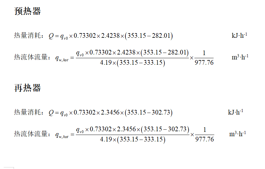
**第二部分,**预热器和再热器的热量以及热流体流量,这些的实现是通过调用第一部分的天然气流量预测结果并结合相应公式进行计算的出结果,其中输入的开始时间和截止时间同样是为了显示这段时间的热量消耗以及热流体流量的结果
**第三部分,**发电量的预测,其同样需要调用第一部分的天然气流量预测结果并结合计算公式进行输出,输入起始时间与上述类似,同时多加一个框输出㶲
设计思路分析
程序概述
此程序使用Python的Dash框架构建了一个交互式的Web应用,该应用主要功能包括:
- 显示特定时间段内预测的天然气流量。
- 根据天然气流量预测结果,计算并展示预热器和再热器的热量消耗及热流体流量。
- 根据天然气流量预测结果,计算并展示发电量。
第一部分:天然气流量预测
数据加载与预处理
- 使用
pandas库从Excel文件中加载数据,并将包含时间信息的列转换为datetime格式,以便后续的时间序列分析。
布局设计
- 在首页中,用户可以通过日期选择器来指定要查看的起始和结束时间。
- 一个加载动画被设置在图表周围,以提高用户体验,当数据正在加载或更新时显示。
- 当用户点击"前往第二页"或"前往第三页"的按钮时,将跳转到相应的页面。
回调函数
- 当用户更改日期选择器中的日期时,触发一个回调函数。该函数将根据所选日期范围筛选数据,并使用这些数据绘制天然气流量的折线图。
第二部分:预热器和再热器的热量及热流体流量计算
布局设计
- 用户可以再次选择起始和结束时间,以查看预热器和再热器在这段时间内的热量消耗和热流体流量。
- 页面中包含了表格,用于展示设备的一些关键参数,如入口温度、入口压力等。
- 两个图表分别展示预热器和再热器的热量消耗以及热流体流量。
计算逻辑
- 这部分利用之前预测的天然气流量数据,结合一些物理公式计算出预热器和再热器的热量消耗以及热流体流量。
- 假设您已经有一个函数或模型能够接受天然气流量作为输入,并返回热量消耗和热流体流量。
- 每个图表将根据用户选择的时间段更新,展示相关的数据。
第三部分:发电量预测
布局设计
- 用户可以再次选择起始和结束时间,以查看这段时间内的发电量预测。
- 页面中包含了四个膨胀机的关键参数表,每个膨胀机都有其各自的入口温度、入口压力、出口温度和出口压力。
- 包含一个图表展示总发电量随时间的变化情况。
计算逻辑
- 这部分同样基于预测的天然气流量数据,通过一些假设和计算公式得到各个膨胀机的发电量。
- 每个膨胀机的发电量计算可能基于不同的效率模型或公式。
- 总发电量由所有膨胀机的发电量累加得出。
- 图表将根据用户选择的时间段更新,展示发电量的变化趋势。
技术细节
- 使用
dash和dash_bootstrap_components来构建界面。 - 使用
pandas进行数据处理。 - 使用
plotly进行数据可视化。 - 使用回调机制来响应用户的交互行为,例如日期选择器的变化等。
设计要点
- 使用
dash和dash_bootstrap_components来构建界面。 - 使用
pandas进行数据处理。 - 使用
plotly进行数据可视化。 - 使用回调机制来响应用户的交互行为,如日期选择器的变化等。
总结
整个程序设计围绕着天然气流量预测的核心展开,通过一系列的计算逻辑,逐步展示了从流量预测到能量转换的全过程。用户可以通过简单的界面操作获得不同时间段内的关键指标信息。
具体代码展示
加载数据并处理时间
# 加载数据并处理时间列
df = pd.read_excel('data.xlsx', engine='openpyxl')
df['datetime'] = pd.to_datetime(df['时间'])
数据加载与时间处理
- 数据加载:
-
- 使用Pandas库的
read_excel函数从一个名为data.xlsx的Excel文件中读取数据。 - 参数
engine='openpyxl'指定了使用openpyxl作为解析Excel文件的引擎。
- 使用Pandas库的
- 时间列处理:
-
- 将DataFrame中的"时间"列转换为
datetime格式,以便后续能够基于日期进行筛选操作。 - 使用Pandas提供的
to_datetime函数完成这一转换。
- 将DataFrame中的"时间"列转换为
首页布局定义
# 定义首页布局
index_page = dbc.Container([
    #标题元素定义
    dbc.Row([
        dbc.Col(html.H1("天然气流量折线图", className='text-center text-primary mb-4'), width=12)
    ], justify="center"
    #时间选择器(起始时间终止时间)
    dbc.Row([
        dbc.Col(dcc.DatePickerRange(
            id='date-picker-range',
            min_date_allowed=df['datetime'].min(),
            max_date_allowed=df['datetime'].max(),
            initial_visible_month=df['datetime'].min(),
            start_date=df['datetime'].min(),
            end_date=df['datetime'].max(),
            className="mt-4"
        ), width={'size': 6, 'offset': 3})
    ], align="center"),
    //graph-with-slider天然气流量可视化图表
    dbc.Row([
        dbc.Col(dcc.Loading(
            dcc.Graph(id='graph-with-slider'),
            type='circle'
        ), width=12)
    ]),
    dbc.Row([
        dbc.Col(dbc.Button('前往第二页', id='go-to-page-2', n_clicks=0, color="primary", className="mt-4"), width=12)
    ], justify="center"),
    dbc.Row([
        dbc.Col(dbc.Button('前往第三页', id='go-to-page-3', n_clicks=0, color="primary", className="mt-4"), width=12)
    ], justify="center")
], fluid=True, className="p-4")
首页图表的可视化函数
# 更新首页图表的数据(graph-with-slider的数据计算流程)
@app.callback(
    Output('graph-with-slider', 'figure'),
    [
        Input('date-picker-range', 'start_date'),
        Input('date-picker-range', 'end_date')
    ]
)
def update_graph_with_slider(start_date, end_date):
    filtered_df = df[(df['datetime'] >= start_date) & (df['datetime'] <= end_date)]
    fig = go.Figure()
    fig.add_trace(go.Scatter(x=filtered_df['datetime'], y=filtered_df['天然气流量'], mode='lines'))
    fig.update_layout(
        xaxis_title="时间",
        yaxis_title="天然气流量",
        transition_duration=500,
        plot_bgcolor='#f9f9f9',
        paper_bgcolor='#f9f9f9',
        font=dict(color='#333333')
    )
    return fig
首页布局定义
- 容器初始化:
-
- 初始化一个
dbc.Container组件,它作为首页内容的容器。 - 属性
fluid=True确保容器占据整个可用宽度。 className="p-4"添加了内边距,以改善视觉效果。
- 初始化一个
- 标题行:
-
- 创建一个
dbc.Row组件,用于容纳首页的标题。 - 利用
dbc.Col组件创建一个12列宽的列,其中包含了标题文本html.H1。 - 标题文本具有居中对齐、主色调文字和底部外边距等样式。
- 创建一个
- 时间选择器:
-
- 创建一个包含日期选择器的行
dbc.Row。 - 通过
dcc.DatePickerRange组件提供日期范围的选择功能。 - 设置日期选择器的最小和最大允许日期,以及初始可见月份等属性。
- 通过
className="mt-4"添加顶部外边距以改善样式。
- 创建一个包含日期选择器的行
- 图表行:
-
- 创建一行以放置图表
dbc.Row。 - 使用
dcc.Loading组件包装图表,以便在加载数据时显示动画。 - 通过
dcc.Graph(id='graph-with-slider')定义一个图表组件,其数据将通过回调动态更新。
- 创建一行以放置图表
- 导航按钮:
-
- 创建两行各包含一个导航按钮的
dbc.Row组件。 - 每个按钮都设置了ID、颜色、点击次数(初始为0)等属性。
- 按钮被置于居中的列中,以实现居中对齐。
- 创建两行各包含一个导航按钮的
首页图表的可视化函数
- 回调函数定义:
-
- 使用
@app.callback装饰器定义一个回调函数,该函数会在日期选择器的起始或结束日期发生改变时被触发。 - 回调函数的输出是图表组件
graph-with-slider的figure属性,输入是日期选择器的两个Input。
- 使用
- 数据过滤:
-
- 根据用户选择的日期范围,从原始数据
df中筛选出相应的记录。
- 根据用户选择的日期范围,从原始数据
- 图表创建:
-
- 初始化一个新的Plotly图表
go.Figure。 - 向图表中添加一条折线图
go.Scatter,其中x轴为过滤后的日期时间序列,y轴为对应的天然气流量数据。 - 更新图表的布局设置,包括坐标轴标签、过渡动画时长、背景颜色和字体颜色。
- 初始化一个新的Plotly图表
最终,该回调函数返回一个更新后的图表对象,使得Web应用能够在页面上动态更新图表,以反映用户所选日期范围内的天然气流量数据。
第二页布局设计
选取指定数据范围然后绘图
页面二中读取 data.xlsx 表格并进行公式运算最后绘图的过程如下:
- 数据加载:
-
- 使用
pandas从data.xlsx文件中读取数据,并将其存储在名为df的 DataFrame 中。 - 数据中的时间列被转换成 Python 的 datetime 对象,并命名为
datetime。
- 使用
- 数据过滤:
-
- 当用户通过
dcc.DatePickerRange选择一个日期范围时,会触发回调函数update_calculations_charts。 - 在该回调函数中,首先根据用户选定的日期范围对 DataFrame 进行筛选,得到一个名为
filtered_df的 DataFrame。
- 当用户通过
- 公式运算:
-
- 在
filtered_df上执行一系列计算,这些计算基于特定的公式:
- 在
-
-
- 预热器热量消耗 (
Q_preheat) 是根据天然气流量乘以常数得到的。 - 预热器热流体流量 (
q_v_hot_preheat) 也是根据热量消耗除以常数后进一步计算得出。 - 再热器热量消耗 (
Q_reheat) 同样是根据天然气流量乘以不同的常数得到。 - 再热器热流体流量 (
q_v_hot_reheat) 计算方法与预热器类似。
- 预热器热量消耗 (
-
- 图表绘制:
-
- 使用
plotly.graph_objects模块创建四个不同的图表:
- 使用
-
-
- 预热器热量消耗图表 (
fig_preheat_heat_consumption)。 - 预热器热流体流量图表 (
fig_preheat_fluid_flow)。 - 再热器热量消耗图表 (
fig_reheat_heat_consumption)。 - 再热器热流体流量图表 (
fig_reheat_fluid_flow)。
- 预热器热量消耗图表 (
-
-
- 每个图表都使用
go.Scatter创建,并设置了一些共同的布局样式。
- 每个图表都使用
- 回调返回:
-
- 回调函数最终返回这四个图表对象,它们将在页面上展示给用户。
这些计算是基于天然气流量和其他物理参数进行的,比如温度和压力等。计算的目的是为了估计预热器和再热器在不同时间点上的热量消耗以及相关的热流体流量。
具体计算步骤
# 定义第二页布局
page_2_layout = dbc.Container([
    dbc.Row([
        //第二页标题定义
        dbc.Col(html.H1("天然气流量计算器", className='text-center text-primary mb-4'), width=12)
    ], justify="center"),
    dbc.Row([
        //时间选择器
        dbc.Col(dcc.DatePickerRange(
            id='date-picker-range-page-2',
            min_date_allowed=df['datetime'].min(),
            max_date_allowed=df['datetime'].max(),
            initial_visible_month=df['datetime'].min(),
            start_date=df['datetime'].min(),
            end_date=df['datetime'].max(),
            className="mt-4"
        ), width={'size': 6, 'offset': 3})
    ], align="center"),
    dbc.Row([
        //预热器再热器参数+数值
        dbc.Col(dbc.Table.from_dataframe(pd.DataFrame({
            '参数': ['入口温度', '入口压力', '出口温度', '出口压力'],
            '数值': [8.86, 3.62, 'N/A', 1]
        }), striped=True, bordered=True, hover=True), width=12)
    ], className="mt-4"),
    //表格具体数值对应
    dbc.Row([
        dbc.Col(dcc.Graph(id='preheater-heat-consumption-graph'), width=6),
        dbc.Col(dcc.Graph(id='preheater-fluid-flow-graph'), width=6)
    ], className="mt-4"),
    dbc.Row([
        dbc.Col(dcc.Graph(id='reheater-heat-consumption-graph'), width=6),
        dbc.Col(dcc.Graph(id='reheater-fluid-flow-graph'), width=6)
    ], className="mt-4"),
    //超链接
    dbc.Row([
        dbc.Col(dbc.Button('前往第二页', id='go-to-page-2', n_clicks=0, color="primary", className="mt-4"), width=12)
    ], justify="center"),
    dbc.Row([
        dbc.Col(dbc.Button('前往第三页', id='go-to-page-3', n_clicks=0, color="primary", className="mt-4"), width=12)
    ], justify="center")
], fluid=True, className="p-4")
更新第二页图表的计算数据用于画图
# 更新第二页图表的数据
//标明输入输出表格信息
@app.callback(
    [
        Output('preheater-heat-consumption-graph', 'figure'),
        Output('preheater-fluid-flow-graph', 'figure'),
        Output('reheater-heat-consumption-graph', 'figure'),
        Output('reheater-fluid-flow-graph', 'figure')
    ],
    [
        Input('date-picker-range-page-2', 'start_date'),
        Input('date-picker-range-page-2', 'end_date')
    ]
)
//具体计算函数
def update_calculations_charts(start_date, end_date):
    filtered_df = df[(df['datetime'] >= start_date) & (df['datetime'] <= end_date)]

    # 保留原有逻辑
    filtered_df['Q_preheat'] = filtered_df['天然气流量'] * 0.73302 * 2.4238 * (353.15 - 282.01)
    filtered_df['q_v_hot_preheat'] = (filtered_df['Q_preheat'] / (4.19 * (353.15 - 333.15))) * (1 / 977.76)
    filtered_df['Q_reheat'] = filtered_df['天然气流量'] * 0.73302 * 2.3456 * (353.15 - 302.73)
    filtered_df['q_v_hot_reheat'] = (filtered_df['Q_reheat'] / (4.19 * (353.15 - 333.15))) * (1 / 977.76)

    # 构建图表
    fig_preheat_heat_consumption = go.Figure()
    fig_preheat_heat_consumption.add_trace(go.Scatter(x=filtered_df['datetime'], y=filtered_df['Q_preheat'], mode='lines'))
    fig_preheat_heat_consumption.update_layout(title="预热器热量消耗")

    fig_preheat_fluid_flow = go.Figure()
    fig_preheat_fluid_flow.add_trace(go.Scatter(x=filtered_df['datetime'], y=filtered_df['q_v_hot_preheat'], mode='lines'))
    fig_preheat_fluid_flow.update_layout(title="预热器热流体流量")

    fig_reheat_heat_consumption = go.Figure()
    fig_reheat_heat_consumption.add_trace(go.Scatter(x=filtered_df['datetime'], y=filtered_df['Q_reheat'], mode='lines'))
    fig_reheat_heat_consumption.update_layout(title="再热器热量消耗")

    fig_reheat_fluid_flow = go.Figure()
    fig_reheat_fluid_flow.add_trace(go.Scatter(x=filtered_df['datetime'], y=filtered_df['q_v_hot_reheat'], mode='lines'))
    fig_reheat_fluid_flow.update_layout(title="再热器热流体流量")

    # 共同样式
    common_layout = {
        'xaxis_title': "时间",
        'yaxis_title': "数值",
        'transition_duration': 500,
        'plot_bgcolor': '#f9f9f9',
        'paper_bgcolor': '#f9f9f9',
        'font': dict(color='#333333')
    }
    fig_preheat_heat_consumption.update_layout(**common_layout)
    fig_preheat_fluid_flow.update_layout(**common_layout)
    fig_reheat_heat_consumption.update_layout(**common_layout)
    fig_reheat_fluid_flow.update_layout(**common_layout)

    return fig_preheat_heat_consumption, fig_preheat_fluid_flow, fig_reheat_heat_consumption, fig_reheat_fluid_flow
本段代码实现了用于展示天然气流量数据的交互式Web应用的第二页布局及图表数据更新功能。
第二页布局定义
- 容器初始化:
-
- 初始化一个
dbc.Container组件来包含第二页的所有内容。 - 属性
fluid=True确保容器占据整个可用宽度。 className="p-4"添加了内边距以改善视觉效果。
- 初始化一个
- 标题行:
-
- 创建一个
dbc.Row组件,用于容纳第二页的标题。 - 利用
dbc.Col组件创建一个12列宽的列,其中包含了标题文本html.H1。 - 标题文本具有居中对齐、主色调文字和底部外边距等样式。
- 创建一个
- 时间选择器:
-
- 创建一个包含日期选择器的行
dbc.Row。 - 通过
dcc.DatePickerRange组件提供日期范围的选择功能。 - 设置日期选择器的最小和最大允许日期,以及初始可见月份等属性。
- 通过
className="mt-4"添加顶部外边距以改善样式。
- 创建一个包含日期选择器的行
- 参数表格行:
-
- 创建一行以展示一个表格
dbc.Row。 - 使用
dbc.Table组件展示预热器和再热器的相关参数及其数值。 - 表格样式包括交替行颜色、边框和悬停效果。
- 创建一行以展示一个表格
- 图表行:
-
- 创建多行以放置四个不同的图表
dbc.Row。 - 每个图表都使用
dcc.Graph组件,并被包装在dcc.Loading组件中以显示加载动画。 - 图表按照预热器和再热器的热量消耗和热流体流量分别展示。
- 每个图表占用半个宽度,通过CSS类名设置顶部外边距。
- 创建多行以放置四个不同的图表
- 导航按钮:
-
- 创建两行各包含一个导航按钮的
dbc.Row组件。 - 每个按钮都设置了ID、颜色、点击次数(初始为0)等属性。
- 按钮被置于居中的列中,以实现居中对齐。
- 创建两行各包含一个导航按钮的
第二页图表的数据更新功能
- 回调函数定义:
-
- 使用
@app.callback装饰器定义一个回调函数,该函数会在日期选择器的起始或结束日期发生改变时被触发。 - 回调函数的输出是四个图表组件的
figure属性,输入是日期选择器的两个Input。
- 使用
- 数据过滤:
-
- 根据用户选择的日期范围,从原始数据
df中筛选出相应的记录。
- 根据用户选择的日期范围,从原始数据
- 计算逻辑:
-
- 对筛选后的数据进行一系列计算,以确定预热器和再热器的热量消耗和热流体流量。
- 计算公式考虑了特定的常数和温度差值。
- 图表构建:
-
- 对于每个图表,初始化一个新的Plotly图表
go.Figure。 - 向图表中添加一条折线图
go.Scatter,其中x轴为过滤后的日期时间序列,y轴为对应的计算结果。 - 更新图表的布局设置,包括坐标轴标签、过渡动画时长、背景颜色和字体颜色。
- 每个图表都设定了一个特定的标题。
- 对于每个图表,初始化一个新的Plotly图表
最终,该回调函数返回四个更新后的图表对象,使得Web应用能够在页面上动态更新图表,以反映用户所选日期范围内预热器和再热器的热量消耗和热流体流量数据。
第三页布局
# 定义第三页布局
page_3_layout = dbc.Container([
    # 使用居中的标题
    dbc.Row([
        dbc.Col(html.H1("发电量预测", className='text-center text-primary mb-4'), width=12)
    ], justify="center"),
    # 日期选择器
    dbc.Row([
        dbc.Col(dcc.DatePickerRange(
            id='date-picker-range-page-3',
            min_date_allowed=df['datetime'].min(),
            max_date_allowed=df['datetime'].max(),
            initial_visible_month=df['datetime'].min(),
            start_date=df['datetime'].min(),
            end_date=df['datetime'].max(),
            className="mt-4"
        ), width={'size': 6, 'offset': 3})
    ], align="center"),
    # 表格容器
    dbc.Row([
        dbc.Col(html.Div([
            html.H5("膨胀机I", className='mb-2'),
            dbc.Table.from_dataframe(pd.DataFrame({
                '参数': ['入口温度', '入口压力', '出口温度', '出口压力'],
                '数值': [353.15, 3.62, 302.73, 1.9]
            }), striped=True, bordered=True, hover=True, responsive=True, id='static-table-turbine-I'),
            html.P("注: H为发电时间, h; 发电量单位 kWh.", className='small mt-2'),
            html.Div(id='table-turbine-I')
        ]), width=3),
        dbc.Col(html.Div([
            html.H5("膨胀机II", className='mb-2'),
            dbc.Table.from_dataframe(pd.DataFrame({
                '参数': ['入口温度', '入口压力', '出口温度', '出口压力'],
                '数值': [353.15, 1.90, 302.73, 1]
            }), striped=True, bordered=True, hover=True, responsive=True, id='static-table-turbine-II'),
            html.P("注: H为发电时间, h; 发电量单位 kWh.", className='small mt-2'),
            html.H5("发电量", className='mb-2'),
            html.Div(id='table-turbine-II')
        ]), width=3),
        dbc.Col(html.Div([
            html.H5("膨胀机III", className='mb-2'),
            dbc.Table.from_dataframe(pd.DataFrame({
                '参数': ['入口温度', '入口压力', '出口温度', '出口压力'],
                '数值': [353.15, 3.62, 302.73, 1.9]
            }), striped=True, bordered=True, hover=True, responsive=True, id='static-table-turbine-III'),
            html.P("注: H为发电时间, h; 发电量单位 kWh.", className='small mt-2'),
            html.H5("发电量", className='mb-2'),
            html.Div(id='table-turbine-III')
        ]), width=3),
        dbc.Col(html.Div([
            html.H5("膨胀机IV", className='mb-2'),
            dbc.Table.from_dataframe(pd.DataFrame({
                '参数': ['入口温度', '入口压力', '出口温度', '出口压力'],
                '数值': [353.15, 1.90, 302.73, 1]
            }), striped=True, bordered=True, hover=True, responsive=True, id='static-table-turbine-IV'),
            html.P("注: H为发电时间, h; 发电量单位 kWh.", className='small mt-2'),
            html.H5("发电量", className='mb-2'),
            html.Div(id='table-turbine-IV')
        ]), width=3),
    ], className="mt-4"),
    # 发电量图表行
    dbc.Row([
        dbc.Col(dcc.Graph(id='total-electricity-generation-graph'), width=12)
    ], className="mt-4"),
    # 前往第二页的按钮
    dbc.Row([
        dbc.Col(dbc.Button('前往第二页', id='go-to-page-2', n_clicks=0, color="primary", className="mt-4"), width=12)
    ], justify="center"),
    # 前往第四页的按钮
    dbc.Row([
        dbc.Col(dbc.Button('前往第四页', id='go-to-page-4', n_clicks=0, color="primary", className="mt-4"), width=12)
    ], justify="center")
], fluid=True, className=f"p-4 bg-light rounded shadow-sm")
第三页具体计算函数
# 回调函数,用于更新总发电量图表
@app.callback(
    Output('total-electricity-generation-graph', 'figure'),  # 输出图表
    [
        Input('date-picker-range-page-3', 'start_date'),  # 输入起始日期
        Input('date-picker-range-page-3', 'end_date')  # 输入结束日期
    ]
)
def update_total_electricity_generation(start_date, end_date):
    # 过滤 DataFrame 以匹配所选日期范围
    filtered_df = df[(df['datetime'] >= start_date) & (df['datetime'] <= end_date)]

    # 计算各组件的发电量
    filtered_df['N1'] = 2 * (filtered_df['天然气流量'] / 2) * 0.73302 * (994.97 - 888.73) / 3600 * (0.8 - 0.00005) * 0.95 * 1
    filtered_df['N2'] = 2 * (filtered_df['天然气流量'] / 2) * 0.73302 * (1007.1 - 897.77) / 3600 * (0.8 - 0.00005) * 0.95 * 1

    # 计算总发电量
    filtered_df['total_electricity_generation'] = filtered_df['N1'] + filtered_df['N2']

    # 创建总发电量图表
    fig = go.Figure()
    fig.add_trace(go.Scatter(x=filtered_df['datetime'], y=filtered_df['total_electricity_generation'], mode='lines', name='Total Electricity Generation'))
    fig.update_layout(
        xaxis_title="时间",
        yaxis_title="总发电量 (kWh)",
        transition_duration=500,
        plot_bgcolor='#f9f9f9',
        paper_bgcolor='#f9f9f9',
        font=dict(color='#333333')
    )

    # 返回图表
    return fig
定义了一个Dash应用中的第三页布局,其中包括了标题、日期选择器、多个表格、一个图表以及导航按钮。此外,还定义了一个回调函数用于更新总发电量的图表数据。
第三页布局定义
- 容器初始化:
-
- 使用
dbc.Container组件初始化一个容器来容纳第三页的所有内容。 - 设置
fluid=True使容器占据整个视口宽度。 className属性为容器添加了内边距、背景色、圆角和阴影等样式。
- 使用
- 标题行:
-
- 创建一个
dbc.Row组件来容纳页面标题。 - 在
dbc.Col中放置了一个html.H1元素作为标题"发电量预测"。 - 设置标题样式使其居中、使用主色调文字并添加底部外边距。
- 创建一个
- 日期选择器:
-
- 创建一行以放置日期选择器
dbc.Row。 - 日期选择器
dcc.DatePickerRange允许用户选择一个日期范围。 - 设置日期选择器的最小、最大允许日期、初始可见月份等属性。
- 日期选择器居中显示,宽度占6列,左侧有3列的空隙。
- 创建一行以放置日期选择器
- 表格容器:
-
- 创建一行以容纳四个表格
dbc.Row。 - 每个表格展示了膨胀机I到IV的相关参数和数值。
- 每个表格使用
dbc.Table组件从DataFrame创建,并具有条纹、边框、鼠标悬停效果和响应式设计。 - 每个表格占3列宽度,并包含相关注释和一个空的
html.Div,可能是为了后续添加动态内容。
- 创建一行以容纳四个表格
- 发电量图表行:
-
- 创建一行以放置总发电量图表
dbc.Row。 - 使用
dcc.Graph组件创建一个空图表,并设置其ID以便动态更新。 - 图表宽度占12列。
- 创建一行以放置总发电量图表
- 导航按钮:
-
- 创建两行各包含一个导航按钮
dbc.Row。 - 每个按钮都有ID、颜色、点击次数等属性。
- 按钮被置于居中的列中以实现居中对齐。
- 创建两行各包含一个导航按钮
回调函数
- 回调函数定义:
-
- 使用
@app.callback装饰器定义一个回调函数。 - 当日期选择器的起始或结束日期发生变化时,该函数会被触发。
- 函数的输出是
total-electricity-generation-graph图表的figure属性。 - 输入是日期选择器的两个
Input。
- 使用
- 数据过滤:
-
- 从原始数据
df中根据用户选择的日期范围筛选数据。 - 过滤条件为
df['datetime'] >= start_date和df['datetime'] <= end_date。
- 从原始数据
- 计算逻辑:
-
- 对筛选后的数据进行计算,以确定膨胀机I和II的发电量
N1和N2。 - 计算公式考虑了特定的常数、天然气流量和温度差值。
- 总发电量
total_electricity_generation为N1和N2之和。
- 对筛选后的数据进行计算,以确定膨胀机I和II的发电量
- 图表构建:
-
- 初始化一个空的
go.Figure对象。 - 添加一条折线图
go.Scatter,其中x轴为过滤后的日期时间序列,y轴为总发电量。 - 更新图表布局,包括坐标轴标签、过渡动画时长、背景颜色和字体颜色。
- 返回图表对象以更新页面上的图表。
- 初始化一个空的
最终,这段代码定义了一个包含标题、日期选择器、表格和图表的页面布局,并定义了一个回调函数来更新图表中的数据,以反映用户所选日期范围内的总发电量数据。
dash页面切换逻辑与回调函数
# 设置Dash应用的主布局
app.layout = html.Div([
    dcc.Location(id='url', refresh=False),
    html.Button('Go to Index Page', id='go-to-index-page', n_clicks=0),
    html.Div(id='page-content')
])
# 处理页面之间的导航
@app.callback(
    Output('url', 'pathname'),
    [Input('go-to-page-2', 'n_clicks'), Input('go-to-page-3', 'n_clicks'), Input('go-to-index-page', 'n_clicks')],
    [State('url', 'pathname')]
)
def navigate_to_page(n_clicks_page_2, n_clicks_page_3, n_clicks_index, pathname):
    ctx = dash.callback_context

    if not ctx.triggered:
        return pathname
    else:
        button_id = ctx.triggered[0]['prop_id'].split('.')[0]

    if button_id == 'go-to-page-2' and pathname != '/page-2':
        return '/page-2'
    elif button_id == 'go-to-page-3' and pathname != '/page-3':
        return '/page-3'
    elif button_id == 'go-to-index-page' and pathname != '/':
        return '/'
    return pathname

# 更新页面内容的回调
@app.callback(Output('page-content', 'children'),
              [Input('url', 'pathname')])
def display_page(pathname):
    if pathname == '/page-2':
        return page_2_layout
    elif pathname == '/page-3':
        return page_3_layout
    else:
        return index_page

# 运行Dash服务器
if __name__ == '__main__':
    app.run_server(debug=True)
这段代码定义了一个Dash应用的基本结构,包括设置主布局、处理页面间的导航以及运行服务器。下面是每个部分的详细解释:
Dash应用主布局设置
- 主布局定义:
-
- 使用
html.Div组件来创建Dash应用的主体布局。 dcc.Location组件用于跟踪和更新URL地址,它是Dash应用中导航的关键组件。html.Button组件创建了一个按钮,用户可以通过点击它回到首页(index page)。html.Div组件用于动态显示不同的页面内容,其ID为page-content。
- 使用
- 导航按钮:
-
- 定义了一个按钮
html.Button,用户可以点击这个按钮回到首页。 - 设置按钮的ID为
go-to-index-page,并初始化点击次数n_clicks为0。
- 定义了一个按钮
- 内容显示区域:
-
- 定义了一个
html.Div组件,其ID为page-content。 - 该组件将根据用户导航至的不同页面路径动态显示相应的页面内容。
- 定义了一个
页面导航处理
- 导航回调函数:
-
- 使用
@app.callback装饰器定义了一个回调函数,用于处理页面间的导航。 - 函数输出为
dcc.Location组件的pathname属性,即URL路径。 - 输入为三个按钮的点击次数:
go-to-page-2、go-to-page-3和go-to-index-page。 - 另一个输入为当前的URL路径状态
State('url', 'pathname')。
- 使用
- 获取触发上下文:
-
- 使用
dash.callback_context来获取触发回调的上下文。 - 如果没有触发事件,则直接返回当前路径
pathname。 - 如果有触发事件,则通过
ctx.triggered[0]['prop_id']来确定哪个按钮触发了回调。
- 使用
- 导航逻辑:
-
- 根据按钮ID判断用户点击的是哪个按钮,并检查当前路径是否需要改变。
- 如果按钮ID对应
go-to-page-2且当前路径不是/page-2,则更新路径为/page-2。 - 类似地,如果按钮ID对应
go-to-page-3且当前路径不是/page-3,则更新路径为/page-3。 - 如果按钮ID对应
go-to-index-page且当前路径不是/,则更新路径为/。 - 如果以上条件都不满足,则保持当前路径不变。
动态页面内容显示
- 页面内容显示回调函数:
-
- 使用
@app.callback装饰器定义了一个回调函数,用于根据当前路径动态显示页面内容。 - 函数输出为
html.Div组件page-content的内容。 - 输入为
dcc.Location组件的pathname属性。
- 使用
- 页面内容更新逻辑:
-
- 根据
pathname的值决定要显示的页面内容。 - 如果路径为
/page-2,则返回page_2_layout作为页面内容。 - 如果路径为
/page-3,则返回page_3_layout作为页面内容。 - 否则,返回
index_page作为首页内容。
- 根据
运行Dash服务器
- 运行服务器:
-
- 使用
if __name__ == '__main__':来确保当脚本被直接运行时才会启动服务器。 - 调用
app.run_server(debug=True)来启动Dash应用服务器。 - 设置
debug=True使得服务器在开发模式下运行,可以实时看到更改效果并获得调试信息。
- 使用
通过这些代码,Dash应用可以实现基本的多页面导航功能,用户可以通过点击按钮在不同页面之间跳转,并且每个页面会有不同的内容展示。
完整代码:
import pandas as pd
import dash
import dash_bootstrap_components as dbc
from dash import dcc, html
from dash.dependencies import Input, Output, State
import plotly.graph_objects as go

# 加载数据并处理时间列
df = pd.read_excel('data.xlsx', engine='openpyxl')
df['datetime'] = pd.to_datetime(df['时间'])

# 初始化Dash应用
app = dash.Dash(__name__, external_stylesheets=[dbc.themes.BOOTSTRAP], suppress_callback_exceptions=True)

# 定义颜色主题
primary_color = '#007BFF'
secondary_color = '#6C757D'
bg_light_color = '#F8F9FA'

# 定义首页布局
index_page = dbc.Container([
    # 使用居中的标题
    dbc.Row([
        dbc.Col(html.H1("天然气流量折线图", className='text-center text-primary mb-4'), width=12)
    ], justify="center"),
    # 日期选择器
    dbc.Row([
        dbc.Col(dcc.DatePickerRange(
            id='date-picker-range',
            min_date_allowed=df['datetime'].min(),
            max_date_allowed=df['datetime'].max(),
            initial_visible_month=df['datetime'].min(),
            start_date=df['datetime'].min(),
            end_date=df['datetime'].max(),
            className="mt-4"
        ), width={'size': 6, 'offset': 3})
    ], align="center"),
    # 图表容器
    dbc.Row([
        dbc.Col(dcc.Loading(
            dcc.Graph(id='graph-with-slider'),
            type='circle'
        ), width=12)
    ], className="mt-4"),
    # 前往第二页的按钮
    dbc.Row([
        dbc.Col(dbc.Button('天然气流量计算器', id='go-to-page-2', n_clicks=0, color="primary", className="mt-4"), width=12)
    ], justify="center"),
    # 前往第三页的按钮
    dbc.Row([
        dbc.Col(dbc.Button('发电量预测', id='go-to-page-3', n_clicks=0, color="primary", className="mt-4"), width=12)
    ], justify="center")
], fluid=True, className=f"p-4 bg-light rounded shadow-sm")

# 更新图表的样式
graph_container_style = {
    "height": "600px",
    "margin-top": "2rem",
    "padding": "1rem",
    "border": "1px solid #eaeaea",
    "border-radius": "5px",
}
index_page.children[2].children[0].style = graph_container_style

# 定义第二页布局
page_2_layout = dbc.Container([
    # 使用居中的标题
    dbc.Row([
        dbc.Col(html.H1("天然气流量计算器", className='text-center text-primary mb-4'), width=12)
    ], justify="center"),
    # 日期选择器
    dbc.Row([
        dbc.Col(dcc.DatePickerRange(
            id='date-picker-range-page-2',
            min_date_allowed=df['datetime'].min(),
            max_date_allowed=df['datetime'].max(),
            initial_visible_month=df['datetime'].min(),
            start_date=df['datetime'].min(),
            end_date=df['datetime'].max(),
            className="mt-4"
        ), width={'size': 6, 'offset': 3})
    ], align="center"),
    # 参数表格
    dbc.Row([
        dbc.Col(dbc.Table.from_dataframe(pd.DataFrame({
            '参数': ['入口温度', '入口压力', '出口温度', '出口压力'],
            '数值': [8.86, 3.62, 'N/A', 1]
        }), striped=True, bordered=True, hover=True, responsive=True), width=12)
    ], className="mt-4"),
    # 图表容器
    dbc.Row([
        dbc.Col(dcc.Graph(id='preheater-heat-consumption-graph'), width=6),
        dbc.Col(dcc.Graph(id='preheater-fluid-flow-graph'), width=6)
    ], className="mt-4"),
    dbc.Row([
        dbc.Col(dcc.Graph(id='reheater-heat-consumption-graph'), width=6),
        dbc.Col(dcc.Graph(id='reheater-fluid-flow-graph'), width=6)
    ], className="mt-4"),
    # 前往第二页的按钮
    dbc.Row([
        dbc.Col(dbc.Button('天然气流量计算器', id='go-to-page-2', n_clicks=0, color="primary", className="mt-4"), width=12)
    ], justify="center"),
    # 前往第三页的按钮
    dbc.Row([
        dbc.Col(dbc.Button('发电量预测', id='go-to-page-3', n_clicks=0, color="primary", className="mt-4"), width=12)
    ], justify="center")
], fluid=True, className=f"p-4 bg-light rounded shadow-sm")

# 定义第三页布局
page_3_layout = dbc.Container([
    # 使用居中的标题
    dbc.Row([
        dbc.Col(html.H1("发电量预测", className='text-center text-primary mb-4'), width=12)
    ], justify="center"),
    # 日期选择器
    dbc.Row([
        dbc.Col(dcc.DatePickerRange(
            id='date-picker-range-page-3',
            min_date_allowed=df['datetime'].min(),
            max_date_allowed=df['datetime'].max(),
            initial_visible_month=df['datetime'].min(),
            start_date=df['datetime'].min(),
            end_date=df['datetime'].max(),
            className="mt-4"
        ), width={'size': 6, 'offset': 3})
    ], align="center"),
    # 表格容器
    dbc.Row([
        dbc.Col(html.Div([
            html.H5("膨胀机I", className='mb-2'),
            dbc.Table.from_dataframe(pd.DataFrame({
                '参数': ['入口温度', '入口压力', '出口温度', '出口压力'],
                '数值': [353.15, 3.62, 302.73, 1.9]
            }), striped=True, bordered=True, hover=True, responsive=True, id='static-table-turbine-I'),
            html.P("注: H为发电时间, h; 发电量单位 kWh.", className='small mt-2'),
            html.Div(id='table-turbine-I')
        ]), width=3),
        dbc.Col(html.Div([
            html.H5("膨胀机II", className='mb-2'),
            dbc.Table.from_dataframe(pd.DataFrame({
                '参数': ['入口温度', '入口压力', '出口温度', '出口压力'],
                '数值': [353.15, 1.90, 302.73, 1]
            }), striped=True, bordered=True, hover=True, responsive=True, id='static-table-turbine-II'),
            html.P("注: H为发电时间, h; 发电量单位 kWh.", className='small mt-2'),
            html.Div(id='table-turbine-II')
        ]), width=3),
        dbc.Col(html.Div([
            html.H5("膨胀机III", className='mb-2'),
            dbc.Table.from_dataframe(pd.DataFrame({
                '参数': ['入口温度', '入口压力', '出口温度', '出口压力'],
                '数值': [353.15, 3.62, 302.73, 1.9]
            }), striped=True, bordered=True, hover=True, responsive=True, id='static-table-turbine-III'),
            html.P("注: H为发电时间, h; 发电量单位 kWh.", className='small mt-2'),
            html.Div(id='table-turbine-III')
        ]), width=3),
        dbc.Col(html.Div([
            html.H5("膨胀机IV", className='mb-2'),
            dbc.Table.from_dataframe(pd.DataFrame({
                '参数': ['入口温度', '入口压力', '出口温度', '出口压力'],
                '数值': [353.15, 1.90, 302.73, 1]
            }), striped=True, bordered=True, hover=True, responsive=True, id='static-table-turbine-IV'),
            html.P("注: H为发电时间, h; 发电量单位 kWh.", className='small mt-2'),
            html.Div(id='table-turbine-IV')
        ]), width=3),
    ], className="mt-4"),
    # 发电量图表行
    dbc.Row([
        dbc.Col(dcc.Graph(id='total-electricity-generation-graph'), width=12)
    ], className="mt-4"),
    # 前往第二页的按钮
    dbc.Row([
        dbc.Col(dbc.Button('天然气流量计算器', id='go-to-page-2', n_clicks=0, color="primary", className="mt-4"), width=12)
    ], justify="center"),
], fluid=True, className=f"p-4 bg-light rounded shadow-sm")


# 更新首页图表的数据
@app.callback(
    Output('graph-with-slider', 'figure'),
    [
        Input('date-picker-range', 'start_date'),
        Input('date-picker-range', 'end_date')
    ]
)
def update_graph_with_slider(start_date, end_date):
    filtered_df = df[(df['datetime'] >= start_date) & (df['datetime'] <= end_date)]
    fig = go.Figure()
    fig.add_trace(go.Scatter(x=filtered_df['datetime'], y=filtered_df['天然气流量'], mode='lines'))
    fig.update_layout(
        xaxis_title="时间",
        yaxis_title="天然气流量",
        transition_duration=500,
        plot_bgcolor='#f9f9f9',
        paper_bgcolor='#f9f9f9',
        font=dict(color='#333333')
    )
    return fig

# 更新第二页图表的数据
@app.callback(
    [
        Output('preheater-heat-consumption-graph', 'figure'),
        Output('preheater-fluid-flow-graph', 'figure'),
        Output('reheater-heat-consumption-graph', 'figure'),
        Output('reheater-fluid-flow-graph', 'figure')
    ],
    [
        Input('date-picker-range-page-2', 'start_date'),
        Input('date-picker-range-page-2', 'end_date')
    ]
)
def update_calculations_charts(start_date, end_date):
    filtered_df = df[(df['datetime'] >= start_date) & (df['datetime'] <= end_date)]

    # 保留原有逻辑
    filtered_df['Q_preheat'] = filtered_df['天然气流量'] * 0.73302 * 2.4238 * (353.15 - 282.01)
    filtered_df['q_v_hot_preheat'] = (filtered_df['Q_preheat'] / (4.19 * (353.15 - 333.15))) * (1 / 977.76)
    filtered_df['Q_reheat'] = filtered_df['天然气流量'] * 0.73302 * 2.3456 * (353.15 - 302.73)
    filtered_df['q_v_hot_reheat'] = (filtered_df['Q_reheat'] / (4.19 * (353.15 - 333.15))) * (1 / 977.76)

    # 构建图表
    fig_preheat_heat_consumption = go.Figure()
    fig_preheat_heat_consumption.add_trace(go.Scatter(x=filtered_df['datetime'], y=filtered_df['Q_preheat'], mode='lines'))
    fig_preheat_heat_consumption.update_layout(title="预热器热量消耗")

    fig_preheat_fluid_flow = go.Figure()
    fig_preheat_fluid_flow.add_trace(go.Scatter(x=filtered_df['datetime'], y=filtered_df['q_v_hot_preheat'], mode='lines'))
    fig_preheat_fluid_flow.update_layout(title="预热器热流体流量")

    fig_reheat_heat_consumption = go.Figure()
    fig_reheat_heat_consumption.add_trace(go.Scatter(x=filtered_df['datetime'], y=filtered_df['Q_reheat'], mode='lines'))
    fig_reheat_heat_consumption.update_layout(title="再热器热量消耗")

    fig_reheat_fluid_flow = go.Figure()
    fig_reheat_fluid_flow.add_trace(go.Scatter(x=filtered_df['datetime'], y=filtered_df['q_v_hot_reheat'], mode='lines'))
    fig_reheat_fluid_flow.update_layout(title="再热器热流体流量")

    # 共同样式
    common_layout = {
        'xaxis_title': "时间",
        'yaxis_title': "数值",
        'transition_duration': 500,
        'plot_bgcolor': '#f9f9f9',
        'paper_bgcolor': '#f9f9f9',
        'font': dict(color='#333333')
    }
    fig_preheat_heat_consumption.update_layout(**common_layout)
    fig_preheat_fluid_flow.update_layout(**common_layout)
    fig_reheat_heat_consumption.update_layout(**common_layout)
    fig_reheat_fluid_flow.update_layout(**common_layout)

    return fig_preheat_heat_consumption, fig_preheat_fluid_flow, fig_reheat_heat_consumption, fig_reheat_fluid_flow


# 回调函数,用于更新总发电量图表
@app.callback(
    Output('total-electricity-generation-graph', 'figure'),  # 输出图表
    [
        Input('date-picker-range-page-3', 'start_date'),  # 输入起始日期
        Input('date-picker-range-page-3', 'end_date')  # 输入结束日期
    ]
)
def update_total_electricity_generation(start_date, end_date):
    # 过滤 DataFrame 以匹配所选日期范围
    filtered_df = df[(df['datetime'] >= start_date) & (df['datetime'] <= end_date)]

    # 计算各组件的发电量
    filtered_df['N1'] = 2 * (filtered_df['天然气流量'] / 2) * 0.73302 * (994.97 - 888.73) / 3600 * (0.8 - 0.00005) * 0.95 * 2
    filtered_df['N2'] = 2 * (filtered_df['天然气流量'] / 2) * 0.73302 * (1007.1 - 897.77) / 3600 * (0.8 - 0.00005) * 0.95 * 2

    # 计算总发电量
    filtered_df['total_electricity_generation'] = filtered_df['N1'] + filtered_df['N2']

    # 创建总发电量图表
    fig = go.Figure()
    fig.add_trace(go.Scatter(x=filtered_df['datetime'], y=filtered_df['total_electricity_generation'], mode='lines', name='Total Electricity Generation'))
    fig.update_layout(
        xaxis_title="时间",
        yaxis_title="总发电量 (kWh)",
        transition_duration=500,
        plot_bgcolor='#f9f9f9',
        paper_bgcolor='#f9f9f9',
        font=dict(color='#333333')
    )

    # 返回图表
    return fig

# 设置Dash应用的主布局
app.layout = html.Div([
    dcc.Location(id='url', refresh=False),
    html.Button('Go to Index Page', id='go-to-index-page', n_clicks=0),
    html.Div(id='page-content')
])
# 处理页面之间的导航
@app.callback(
    Output('url', 'pathname'),
    [Input('go-to-page-2', 'n_clicks'), Input('go-to-page-3', 'n_clicks'), Input('go-to-index-page', 'n_clicks')],
    [State('url', 'pathname')]
)
def navigate_to_page(n_clicks_page_2, n_clicks_page_3, n_clicks_index, pathname):
    ctx = dash.callback_context

    if not ctx.triggered:
        return pathname
    else:
        button_id = ctx.triggered[0]['prop_id'].split('.')[0]

    if button_id == 'go-to-page-2' and pathname != '/page-2':
        return '/page-2'
    elif button_id == 'go-to-page-3' and pathname != '/page-3':
        return '/page-3'
    elif button_id == 'go-to-index-page' and pathname != '/':
        return '/'
    return pathname

# 更新页面内容的回调
@app.callback(Output('page-content', 'children'),
              [Input('url', 'pathname')])
def display_page(pathname):
    if pathname == '/page-2':
        return page_2_layout
    elif pathname == '/page-3':
        return page_3_layout
    else:
        return index_page

# 运行Dash服务器
if __name__ == '__main__':
    app.run_server(debug=True)

import numpy as np
import pandas as pd
import tensorflow as tf
from keras.models import Sequential
from keras.layers import LSTM, Dense, Dropout
from sklearn.preprocessing import MinMaxScaler
from sklearn.metrics import mean_squared_error, mean_absolute_error, r2_score, mean_absolute_percentage_error
from keras.callbacks import EarlyStopping, ModelCheckpoint
import matplotlib.pyplot as plt
from pathlib import Path
import os
from matplotlib import rc
from scipy import stats

# 加载和预处理数据
data_file = Path("C:\\Users\\huangshaozheng\\Desktop\\modified_yaodian.xlsx")

try:
    data = pd.read_excel(data_file, parse_dates=['日期'], index_col='日期')
except FileNotFoundError:
    print(f"错误:文件 {data_file} 未找到。")
    exit(1)
except ValueError as e:
    print(f"错误:{e}")
    exit(1)

# 检查数据格式
print(data.head())

# 检测和移除异常值
z = np.abs(stats.zscore(data))
data = data[(z < 3).all(axis=1)]

# 归一化数据
scaler = MinMaxScaler(feature_range=(0, 1))
scaled_data = scaler.fit_transform(data)

# 定义时间窗口大小
window_size = 3

# 创建训练和测试数据集
train_size = int(len(scaled_data) * 0.9)
train_data = scaled_data[:train_size]
test_data = scaled_data[train_size:]

def create_dataset(data, window_size):
    X, y = [], []
    for i in range(len(data) - window_size):
        X.append(data[i:i+window_size])
        y.append(data[i+window_size])
    return np.array(X), np.array(y)

train_X, train_y = create_dataset(train_data, window_size)
test_X, test_y = create_dataset(test_data, window_size)

# 调整数据形状以适应LSTM输入
train_X = train_X.reshape((train_X.shape[0], train_X.shape[1], 1))
test_X = test_X.reshape((test_X.shape[0], test_X.shape[1], 1))

# 建立LSTM模型
model = Sequential()
model.add(LSTM(units=64, return_sequences=True, input_shape=(window_size, 1)))
model.add(Dropout(0.2))
model.add(LSTM(units=64))
model.add(Dropout(0.2))
model.add(Dense(units=1))
optimizer = tf.keras.optimizers.Adam(learning_rate=0.001)
model.compile(optimizer=optimizer, loss='mean_squared_error')

# 定义回调
early_stopping = EarlyStopping(monitor='val_loss', patience=10, restore_best_weights=True)
model_checkpoint = ModelCheckpoint('best_model.keras', monitor='val_loss', save_best_only=True)

# 训练模型
history = model.fit(train_X, train_y, epochs=100, batch_size=256, validation_data=(test_X, test_y), callbacks=[early_stopping, model_checkpoint])

# 加载最佳模型
model = tf.keras.models.load_model('best_model.keras')  # 修改文件名结尾为 .keras

# 进行预测
train_predictions = model.predict(train_X)
test_predictions = model.predict(test_X)

# 评价模型性能(在归一化的数据上)
train_mse = mean_squared_error(train_y, train_predictions)
test_mse = mean_squared_error(test_y, test_predictions)
train_rmse = np.sqrt(train_mse)
test_rmse = np.sqrt(test_mse)
train_mae = mean_absolute_error(train_y, train_predictions)
test_mae = mean_absolute_error(test_y, test_predictions)
train_r2 = r2_score(train_y, train_predictions)
test_r2 = r2_score(test_y, test_predictions)
train_mape = mean_absolute_percentage_error(train_y, train_predictions)
test_mape = mean_absolute_percentage_error(test_y, test_predictions)

# 打印评估指标
print(f'Train MSE: {train_mse:.4f}')
print(f'Test MSE: {test_mse:.4f}')
print(f'Train RMSE: {train_rmse:.4f}')
print(f'Test RMSE: {test_rmse:.4f}')
print(f'Train MAE: {train_mae:.4f}')
print(f'Test MAE: {test_mae:.4f}')
print(f'Train R²: {train_r2:.4f}')
print(f'Test R²: {test_r2:.4f}')
print(f'Train MAPE: {train_mape:.4f}')
print(f'Test MAPE: {test_mape:.4f}')

# 反归一化预测值和实际值
train_predictions_inv = scaler.inverse_transform(train_predictions)
test_predictions_inv = scaler.inverse_transform(test_predictions)
train_actual_inv = scaler.inverse_transform(train_y.reshape(-1, 1))
test_actual_inv = scaler.inverse_transform(test_y.reshape(-1, 1))

# 保存目录
save_dir = "C:\\Users\\huangshaozheng\\Desktop\\姚店-延安"

# 获取对应的日期
train_dates = data.index[window_size-1:train_size]
test_dates = data.index[train_size + window_size - 1:]

print("train_dates的长度:", len(train_dates))
print("test_dates的长度:", len(test_dates))
print("train_actual.flatten()的长度:", len(train_actual_inv.flatten()))
print("test_actual.flatten()的长度:", len(test_actual_inv.flatten()))
print("train_predictions.flatten()的长度:", len(train_predictions_inv.flatten()))
print("test_predictions.flatten()的长度:", len(test_predictions_inv.flatten()))

# 创建DataFrame以保存训练集和测试集的日期和实际流量值
train_actual_df = pd.DataFrame({'日期': train_dates[:len(train_actual_inv.flatten())], '训练集实际流量值': train_actual_inv.flatten()})
test_actual_df = pd.DataFrame({'日期': test_dates[:len(test_actual_inv.flatten())], '测试集实际流量值': test_actual_inv.flatten()})

# 创建DataFrame以保存训练集和测试集的日期和预测流量值
train_predictions_df = pd.DataFrame({'日期': train_dates[:len(train_predictions_inv.flatten())], '训练集预测流量值': train_predictions_inv.flatten()})
test_predictions_df = pd.DataFrame({'日期': test_dates[:len(test_predictions_inv.flatten())], '测试集预测流量值': test_predictions_inv.flatten()})

# 确保保存目录存在,如果不存在则创建
os.makedirs(save_dir, exist_ok=True)

# 构建保存文件的完整路径
train_actual_file = os.path.join(save_dir, 'train_actual_flow.xlsx')
test_actual_file = os.path.join(save_dir, 'test_actual_flow.xlsx')
train_predictions_file = os.path.join(save_dir, 'train_predictions_flow.xlsx')
test_predictions_file = os.path.join(save_dir, 'test_predictions_flow.xlsx')

# 将DataFrame写入Excel文件
train_actual_df.to_excel(train_actual_file, index=False)
test_actual_df.to_excel(test_actual_file, index=False)
train_predictions_df.to_excel(train_predictions_file, index=False)
test_predictions_df.to_excel(test_predictions_file, index=False)

print(f'训练集实际流量已保存到 {train_actual_file}')
print(f'测试集实际流量已保存到 {test_actual_file}')
print(f'训练集预测流量已保存到 {train_predictions_file}')
print(f'测试集预测流量已保存到 {test_predictions_file}')

# 设置中文字体
plt.rcParams['font.sans-serif'] = ['SimHei']  # 指定中文字体,这里使用了黑体
plt.rcParams['axes.unicode_minus'] = False    # 解决负号显示为方块的问题

# Visualize the predictions for the training set
plt.figure(figsize=(15, 8))
train_dates = train_dates[:len(train_actual_inv)]
plt.plot(train_dates, train_actual_inv, label='训练集实际流量值')
plt.plot(train_dates, train_predictions_inv, label='训练集预测流量值')
plt.xlabel('日期', fontsize=15)
plt.ylabel('流量值/(m$^3$)', fontsize=15)
plt.title('管道流量数据预测(LSTM模型) - 训练集', fontsize=18)
plt.legend()
plt.xticks(fontsize=12)
plt.yticks(fontsize=12)
plt.show()

# Visualize the predictions for the test set
plt.figure(figsize=(15, 8))
test_dates = test_dates[:len(test_actual_inv.flatten())]  # 确保日期和实际流量值长度一致

plt.plot(test_dates, test_actual_inv.flatten(), label='测试集实际流量值')
plt.plot(test_dates, test_predictions_inv.flatten(), label='测试集预测流量值')
plt.xlabel('日期', fontsize=15)
plt.ylabel('流量值/(m$^3$)', fontsize=15)
plt.title('管道流量数据预测(LSTM模型) - 测试集', fontsize=18)
plt.legend()
plt.xticks(fontsize=12)
plt.yticks(fontsize=12)
plt.show()
1. 导入必要的库
import numpy as np
import pandas as pd
import tensorflow as tf
from keras.models import Sequential
from keras.layers import LSTM, Dense, Dropout
from sklearn.preprocessing import MinMaxScaler
from sklearn.metrics import mean_squared_error, mean_absolute_error, r2_score, mean_absolute_percentage_error
from keras.callbacks import EarlyStopping, ModelCheckpoint
import matplotlib.pyplot as plt
from pathlib import Path
import os
from matplotlib import rc
from scipy import stats
这些是用于数据处理、机器学习、深度学习以及绘图的常用库。
2. 加载和预处理数据
# 加载和预处理数据
data_file = Path("C:\\Users\\huangshaozheng\\Desktop\\modified_yaodian.xlsx")

try:
    data = pd.read_excel(data_file, parse_dates=['日期'], index_col='日期')
except FileNotFoundError:
    print(f"错误:文件 {data_file} 未找到。")
    exit(1)
except ValueError as e:
    print(f"错误:{e}")
    exit(1)

# 检查数据格式
print(data.head())
这里我们尝试从指定路径加载一个Excel文件,并使用Pandas读取该文件。我们确保日期列被正确解析为日期格式,并将该列设置为DataFrame的索引。如果文件不存在或无法正确解析日期,则会打印出错误消息并退出程序。
# 检测和移除异常值
z = np.abs(stats.zscore(data))
data = data[(z < 3).all(axis=1)]
这一部分使用Z-score方法来检测并移除异常值。任何超出平均值3个标准差的数据点都会被视为异常值并被删除。
# 归一化数据
scaler = MinMaxScaler(feature_range=(0, 1))
scaled_data = scaler.fit_transform(data)这里使用MinMaxScaler将数据缩放到0到1之间,这对于神经网络模型来说是非常重要的,因为它们对数据的尺度很敏感。
3. 创建训练和测试数据集
# 定义时间窗口大小
window_size = 3

# 创建训练和测试数据集
train_size = int(len(scaled_data) * 0.9)
train_data = scaled_data[:train_size]
test_data = scaled_data[train_size:]

def create_dataset(data, window_size):
    X, y = [], []
    for i in range(len(data) - window_size):
        X.append(data[i:i+window_size])
        y.append(data[i+window_size])
    return np.array(X), np.array(y)

train_X, train_y = create_dataset(train_data, window_size)
test_X, test_y = create_dataset(test_data, window_size)这部分定义了一个函数create_dataset,它接收原始数据和时间窗口大小作为参数,并返回两个数组:一个包含输入序列(X),另一个包含目标值(y)。这是为了创建监督学习问题,其中每个输入序列对应于下一个时间步的目标值。
4. 准备数据以供LSTM使用
# 调整数据形状以适应LSTM输入
train_X = train_X.reshape((train_X.shape[0], train_X.shape[1], 1))
test_X = test_X.reshape((test_X.shape[0], test_X.shape[1], 1))
LSTM层需要三维输入,因此我们需要调整数据的形状以匹配要求。这里我们增加了一个特征维度,因为我们只有一个特征(即流量值)。
5. 建立LSTM模型
# 建立LSTM模型
model = Sequential()
model.add(LSTM(units=64, return_sequences=True, input_shape=(window_size, 1)))
model.add(Dropout(0.2))
model.add(LSTM(units=64))
model.add(Dropout(0.2))
model.add(Dense(units=1))
optimizer = tf.keras.optimizers.Adam(learning_rate=0.001)
model.compile(optimizer=optimizer, loss='mean_squared_error')
这里我们定义了一个顺序模型,并添加了两个LSTM层以及Dropout层来防止过拟合。最后一层是一个Dense层,用来输出预测结果。我们使用Adam优化器和均方误差损失函数来编译模型。
6. 定义回调函数
# 定义回调
early_stopping = EarlyStopping(monitor='val_loss', patience=10, restore_best_weights=True)
model_checkpoint = ModelCheckpoint('best_model.keras', monitor='val_loss', save_best_only=True)
这里定义了两个回调函数:
EarlyStopping:当验证损失不再改进时停止训练。ModelCheckpoint:保存训练过程中性能最好的模型。
7. 训练模型
# 训练模型
history = model.fit(train_X, train_y, epochs=100, batch_size=256, validation_data=(test_X, test_y), callbacks=[early_stopping, model_checkpoint])
使用训练数据进行模型训练,并通过验证数据集来监控模型的表现。
8. 加载最佳模型
# 加载最佳模型
model = tf.keras.models.load_model('best_model.keras')  # 修改文件名结尾为 .keras
加载之前保存的最佳模型。
9. 进行预测
# 进行预测
train_predictions = model.predict(train_X)
test_predictions = model.predict(test_X)
使用训练好的模型进行预测。
10. 评价模型性能
# 评价模型性能(在归一化的数据上)
...
计算各种评估指标,如均方误差(MSE)、均方根误差(RMSE)、平均绝对误差(MAE)、R²分数和平均绝对百分比误差(MAPE)。
11. 反归一化预测值和实际值
# 反归一化预测值和实际值
...
将预测值和真实值从归一化的状态还原到原始规模。
12. 保存预测结果到Excel文件
# 保存目录
...
创建DataFrame并将预测结果保存到Excel文件中。
13. 绘制预测结果
# 设置中文字体
plt.rcParams['font.sans-serif'] = ['SimHei']  # 指定中文字体,这里使用了黑体
plt.rcParams['axes.unicode_minus'] = False    # 解决负号显示为方块的问题

# Visualize the predictions for the training set
...
设置Matplotlib以支持中文,并绘制训练集和测试集的实际值与预测值的图形。