ml
Course1-Week2:
https://github.com/kaieye/2022-Machine-Learning-Specialization/tree/main/Supervised%20Machine%20Learning%20Regression%20and%20Classification/week2
机器学习笔记(三)
- 1️⃣多元线性回归及矢量化
- [2️⃣特征缩放(Feature Scaling)](#2️⃣特征缩放(Feature Scaling))
- [3️⃣学习率(Learning Rate)](#3️⃣学习率(Learning Rate))
- [4️⃣特征工程(Feature Engineering)](#4️⃣特征工程(Feature Engineering))
- 5️⃣多项式回归
- 6️⃣Scikit-Learn
1️⃣多元线性回归及矢量化
多元线性回归(multiple linear regression)
🎈对于一元线性回归问题,我们只是考虑将 Size 作为 input 的情况来得出房屋的价格。
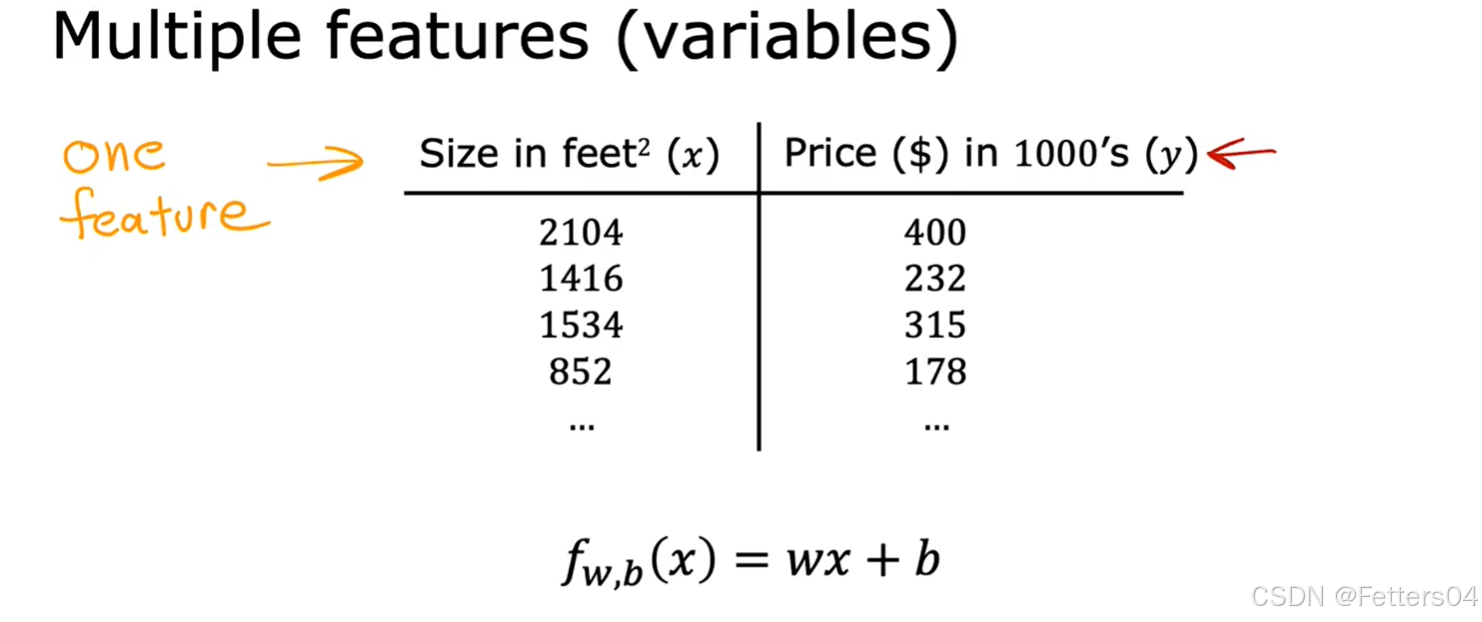
🎈而在现实中考虑房屋价格的因素绝不止有一个,所以我们引入了多维特征(房屋大小,卧室的数量,楼层数量,房屋的年龄)四个维度的特征来得出房价,数据集及说明如下图:
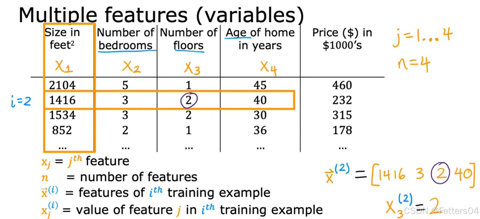
对于这四个维度分别表示为 x 1 , x 2 , x 3 , x 4 x_1,x_2,x_3,x_4 x1,x2,x3,x4 ,为了方便使用向量 x ⃗ \vec x x 来表示,即对于第 i i i 组案例有 x ⃗ ( i ) = ( x 1 ( i ) , x 2 ( i ) , x 3 ( i ) , x 4 ( i ) ) \vec x^{(i)}=({x_1}^{(i)},{x_2}^{(i)},{x_3}^{(i)},{x_4}^{(i)}) x (i)=(x1(i),x2(i),x3(i),x4(i)),所以可以写出这样的线性回归方程:
✨ f w , b ( x ) = w 1 x 1 + w 2 x 2 + w 3 x 3 + w 4 x 4 + b f_{w,b}(x)=w_1x_1+w_2x_2+w_3x_3+w_4x_4+b fw,b(x)=w1x1+w2x2+w3x3+w4x4+b,而对于 w w w也可用向量来表示 w ⃗ = ( w 1 , w 2 , w 3 , w 4 ) \vec w=({w_1},{w_2},{w_3},{w_4}) w =(w1,w2,w3,w4)。
✨ 扩展到 n n n 维,可以得出多元线性回归模型 :
f w ⃗ , b ( x ⃗ ) = w ⃗ ⋅ x ⃗ + b = w 1 x 1 + w 2 x 2 + . . . + w n x n + b \begin{align} f_{\vec w,b}({\vec x}) &= \vec w \cdot \vec x + b \\ &= w_1x_1+w_2x_2+...+w_nx_n+b \end{align} fw ,b(x )=w ⋅x +b=w1x1+w2x2+...+wnxn+b
多元线性回归模型的梯度下降法

矢量化(Vectorization)
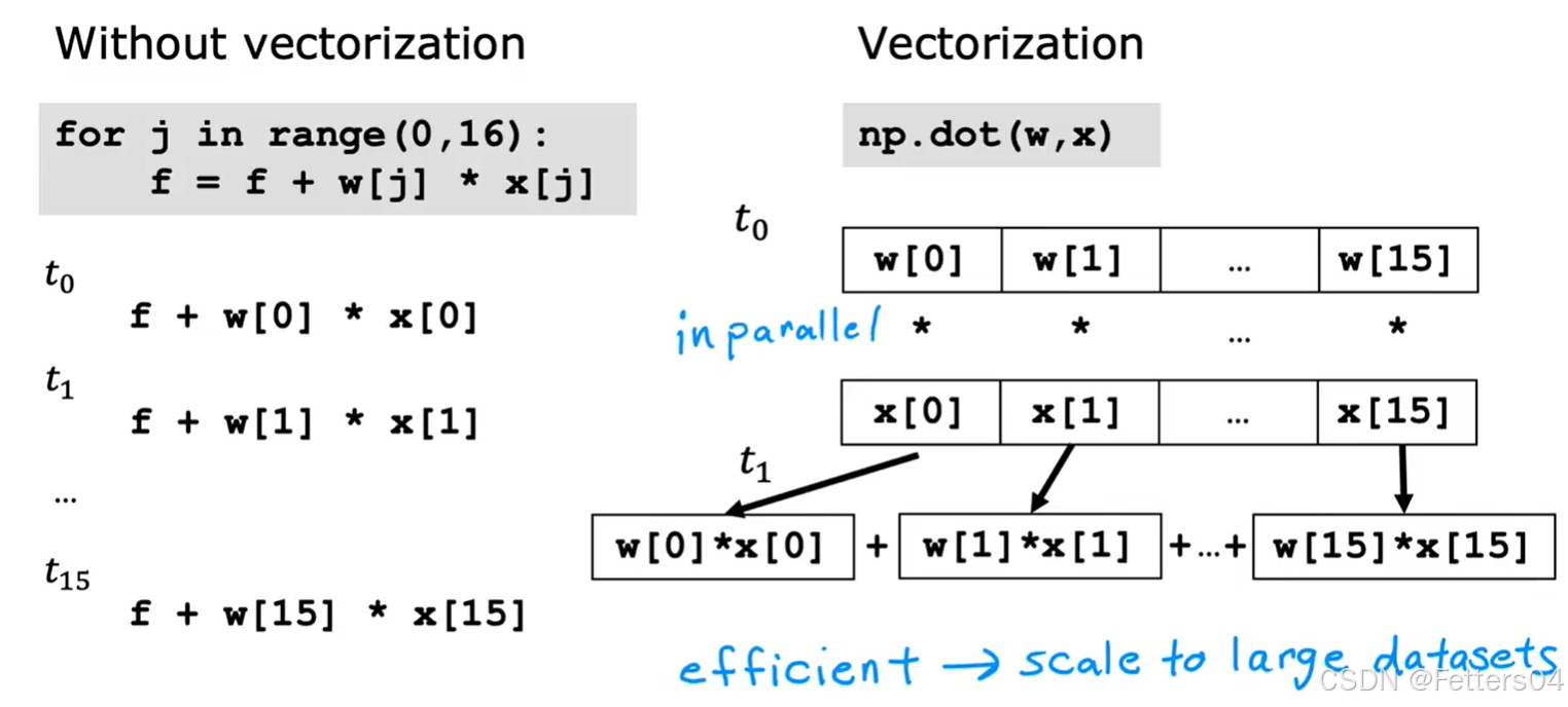
🎈指在数值计算或机器学习中,将循环操作转换为向量或矩阵运算的过程。通过矢量化,可以利用现代处理器的并行计算能力,极大地提升代码的执行效率,尤其是在处理大量数据时。矢量化通常应用于使用 NumPy 或类似库来替代原本的显式循环(for-loop)操作。
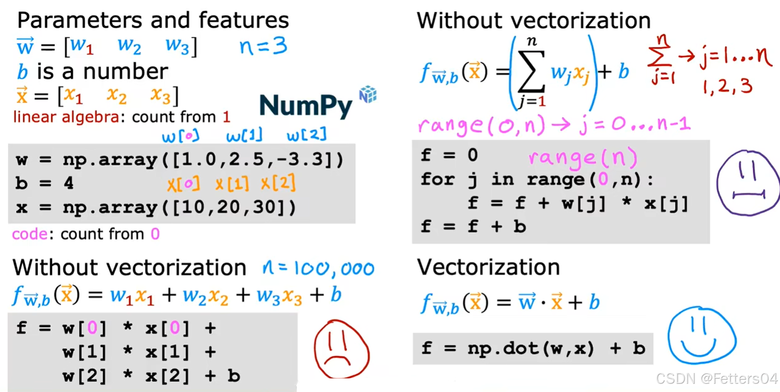
🎈使用 NumPy 的 dot 函数去计算,很好地利用了处理器并行计算的能力,下面通过代码来演示显式循环和矢量化的性能差距。
python
# 引入库
import numpy as np
import time
自定义一个函数用来显式循环计算
python
def my_dot(a, b):
    """
   Compute the dot product of two vectors

    Args:
      a (ndarray (n,)):  input vector
      b (ndarray (n,)):  input vector with same dimension as a

    Returns:
      x (scalar):
    """
    x=0
    for i in range(a.shape[0]):
        x = x + a[i] * b[i]
    return x

print(a.shape[0])
用两个数组 a , b a,b a,b 来模拟一下计算过程
python
np.random.seed(1)
a = np.random.rand(10000000)  # very large arrays
b = np.random.rand(10000000)

tic = time.time()  # capture start time
c = np.dot(a, b)
toc = time.time()  # capture end time

print(f"np.dot(a, b) =  {c:.4f}")
print(f"Vectorized version duration: {1000*(toc-tic):.4f} ms ")

tic = time.time()  # capture start time
c = my_dot(a,b)
toc = time.time()  # capture end time

print(f"my_dot(a, b) =  {c:.4f}")
print(f"loop version duration: {1000*(toc-tic):.4f} ms ")

del(a);del(b)  #remove these big arrays from memory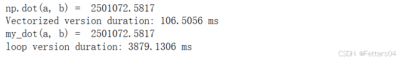
通过演示,可以明显看到两种计算方式之间的性能差距。
2️⃣特征缩放(Feature Scaling)
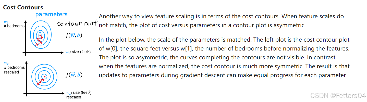
🎈对于不同的特征,例如房屋的大小和卧室数量两种参数,由于房屋的大小这个值是远远大于卧室数量的,如果当选择差不多大的 w w w 时,bedrooms 这个参数对于代价的影响将微乎其微。如果想让两者的影响相当的话可能要让一方选择较大的 w w w,而另一方选择较小的 w w w 去平衡对代价 J J J 的影响。

🎈我们最好还是想让两个参数一视同仁,对代价有着同等的影响。
✨特征缩放起到了这个作用,本质上是将每个特征除以用户选定的一个值,让参数得到 -1 到 1 的范围。

🎊还有两种方法也能达到目的:
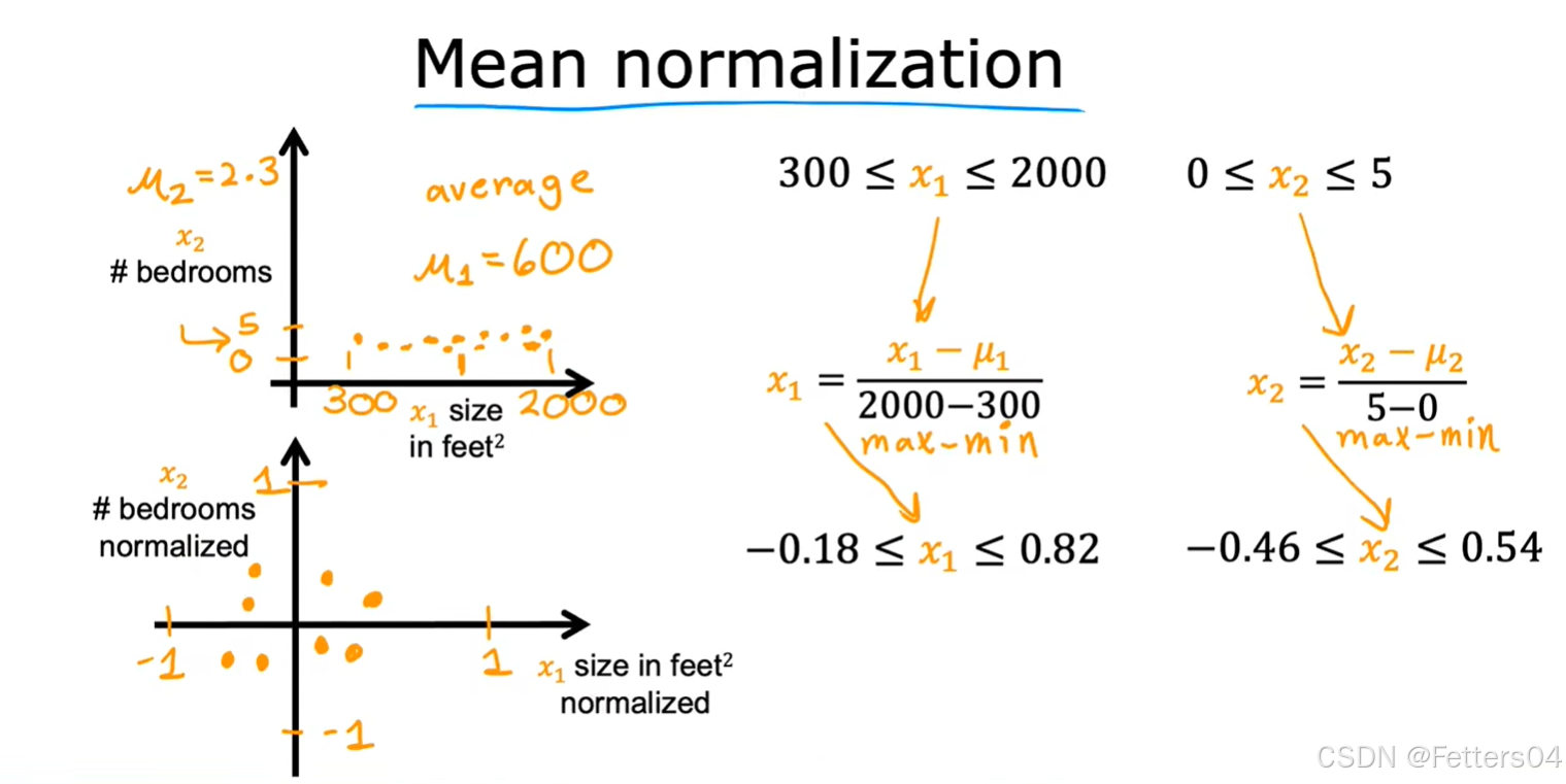
✨均值归一化(Mean normalization):
x i = x i − μ i m a x − m i n , μ i 是所有特征 x 的平均值 x_i= \frac {x_i-\mu_i} {max-min}, \mu_i是所有特征 x 的平均值 xi=max−minxi−μi,μi是所有特征x的平均值
✨Z-score标准化(Z-score normalization):
To implement z-score normalization, adjust your input values as shown in this formula:
x j ( i ) = x j ( i ) − μ j σ j {x_j}^{(i)}= \frac {{x_j}^{(i)}-\mu_j} {\sigma_j} xj(i)=σjxj(i)−μj
where j j j selects a feature or a column in the X matrix. µ j µ_j µj is the mean of all the values for feature(j) and σ j \sigma_j σj is the standard deviation of feature(j).
μ j = 1 m ∑ i = 0 m − 1 x j ( i ) \mu_j=\frac 1 m \sum_{i=0}^{m-1}{x_j}^{(i)} μj=m1i=0∑m−1xj(i)
σ j 2 = 1 m ∑ i = 0 m − 1 ( x j ( i ) − μ j ) 2 {\sigma_j}^2=\frac 1 m \sum_{i=0}^{m-1}({x_j}^{(i)}-\mu_j)^2 σj2=m1i=0∑m−1(xj(i)−μj)2

3️⃣学习率(Learning Rate)
🎈在梯度下降法中可以看到学习率 α \alpha α 的使用,它能控制参数更新的大小,而 α \alpha α 如果太小可能会导致梯度下降代价函数收敛的过程很缓慢;而 α \alpha α 如果过大,很可能会导致代价函数发散。因此选取一个合适的 α \alpha α 对模型来说是很重要的。
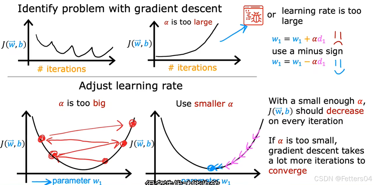
✨寻找 α \alpha α 的一种方法,找一个过小的学习率,逐渐倍数找到个过大的学习率,再从其中寻找合适的 α \alpha α:

4️⃣特征工程(Feature Engineering)
🎈特征工程,是对原始数据进行一系列工程处理,将其提炼为特征,作为输入供算法和模型使用,而之前面对的特征都是线性,然而当面对的特征是非线性的或者是特征的组合又该怎么办?下面开始考虑数据非线性的场景。
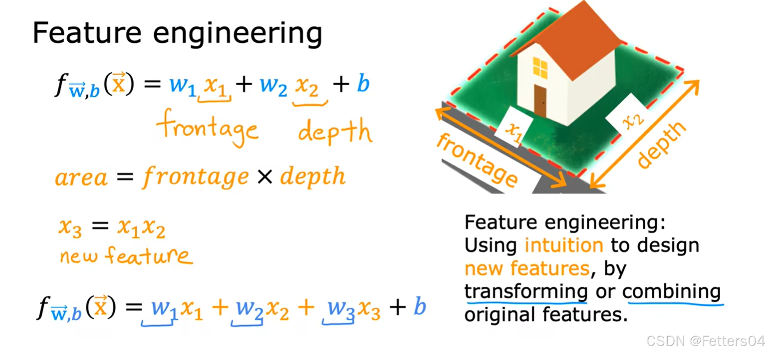
如下是对房价预测的特征方程的考虑,显然都是多项式方程:


5️⃣多项式回归
python
# 导入Lab中的自定义函数和NumPy以及matplotlib 库
import numpy as np
import matplotlib.pyplot as plt
from lab_utils_multi import zscore_normalize_features, run_gradient_descent_feng
np.set_printoptions(precision=2)  # reduced display precision on numpy arrays
🎈我们开始尝试用已知的知识去拟合非线性曲线,例如: y = 1 + x 2 y=1+x^2 y=1+x2 。
对于一个有着平方关系的数据 y y y ,使用线性回归去拟合:
python
# create target data
x = np.arange(0, 20, 1)
y = 1 + x**2
X = x.reshape(-1, 1)

model_w,model_b = run_gradient_descent_feng(X,y,iterations=1000, alpha = 1e-2)

plt.scatter(x, y, marker='x', c='r', label="Actual Value"); plt.title("no feature engineering")
plt.plot(x,X@model_w + model_b, label="Predicted Value");  plt.xlabel("X"); plt.ylabel("y"); plt.legend(); plt.show()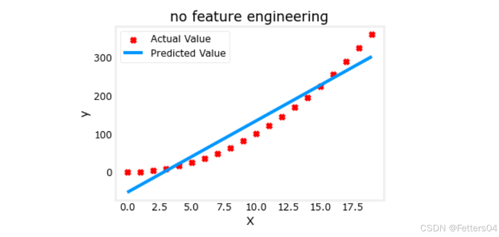
由此可见效果确实不太好,可以需要一个类似 y = w 0 x 0 2 + b y=w_0x_0^2+b y=w0x02+b 的曲线,或者一个多项式特征。如果使用特征工程将 x x x 换为 x 2 x^2 x2 的话看看效果会不会更好。
py
# create target data
x = np.arange(0, 20, 1)
y = 1 + x**2

# Engineer features
X = x**2      #<-- added engineered feature
py
X = X.reshape(-1, 1)  #X should be a 2-D Matrix
model_w,model_b = run_gradient_descent_feng(X, y, iterations=10000, alpha = 1e-5)

plt.scatter(x, y, marker='x', c='r', label="Actual Value"); plt.title("Added x**2 feature")
plt.plot(x, np.dot(X,model_w) + model_b, label="Predicted Value"); plt.xlabel("x"); plt.ylabel("y"); plt.legend(); plt.show()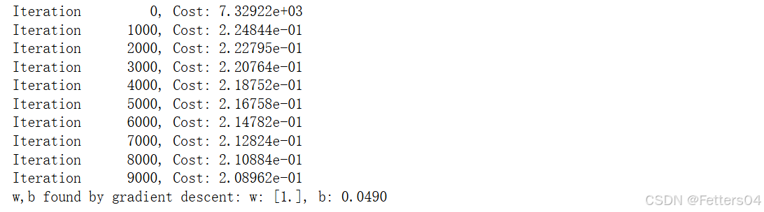
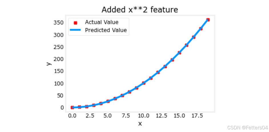
🎉我们获得了一个很好的拟合曲线, y = 1 ∗ x 0 2 + 0.049 y=1*x_0^2+0.049 y=1∗x02+0.049,非常接近目标 y = 1 ∗ x 0 2 + 1 y=1*x_0^2+1 y=1∗x02+1,如果迭代更久效果可能会更好。
✨当对于不是很明显的特征关系,我们可以尝试添加各种潜在的特征来找到一个最合适的拟合曲线,这就是特征工程。我们也许会找到类似 y = w 0 x 0 + w 1 x 1 2 + w 2 x 2 3 + b y=w_0x_0+w_1x_1^2+w_2x_2^3+b y=w0x0+w1x12+w2x23+b 这种形式。如果对于数据集有着明显不同规模的尺寸,别忘了我们还有特征缩放,让每个特征的影响大致不差,并且可以加速梯度下降的过程同时收敛各个参数。
6️⃣Scikit-Learn
官网:https://scikit-learn.org/stable/index.html
🎈Scikit-learn 是一个强大开源的机器学习 Python 库,它建立在 NumPy、SciPy 和 Matplotlib 之上,提供了大量的机器学习算法和工具,用于机器学习和数据分析。它包含了一系列简单易用且高效的工具,用于分类、回归、聚类、降维、模型选择和预处理等。
下面来利用 Scikit-Learn 使用梯度下降实现线性回归。
py
# You will utilize functions from scikit-learn as well as matplotlib and NumPy.
import numpy as np
np.set_printoptions(precision=2)
from sklearn.linear_model import LinearRegression, SGDRegressor
from sklearn.preprocessing import StandardScaler
from lab_utils_multi import  load_house_data
import matplotlib.pyplot as plt
dlblue = '#0096ff'; dlorange = '#FF9300'; dldarkred='#C00000'; dlmagenta='#FF40FF'; dlpurple='#7030A0';
plt.style.use('./deeplearning.mplstyle')
Scikit-learn 有一个梯度下降回归模型 sklearn.linear_model.SGDRegressor,该模型在标准化输入时表现最佳。而 sklearn.preprocessing.StandardScaler 可以实现 Z-score 标准化。
py
# Load the data set
X_train, y_train = load_house_data()
X_features = ['size(sqft)','bedrooms','floors','age']
使用 sklearn.preprocessing.StandardScaler 将训练集标准化
py
scaler = StandardScaler()
X_norm = scaler.fit_transform(X_train)
print(f"Peak to Peak range by column in Raw        X:{np.ptp(X_train,axis=0)}")
print(f"Peak to Peak range by column in Normalized X:{np.ptp(X_norm,axis=0)}")
使用 sklearn.linear_model.SGDRegressor 创建并拟合回归模型。
py
sgdr = SGDRegressor(max_iter=1000)
sgdr.fit(X_norm, y_train)
print(sgdr)
print(f"number of iterations completed: {sgdr.n_iter_}")
对比一下之前的 Lab 的模型参数
py
b_norm = sgdr.intercept_
w_norm = sgdr.coef_
print(f"model parameters:                   w: {w_norm}, b:{b_norm}")
print(f"model parameters from previous lab: w: [110.56 -21.27 -32.71 -37.97], b: 363.16")
做出预测
py
# make a prediction using sgdr.predict()
y_pred_sgd = sgdr.predict(X_norm)
# make a prediction using w,b.
y_pred = np.dot(X_norm, w_norm) + b_norm
print(f"prediction using np.dot() and sgdr.predict match: {(y_pred == y_pred_sgd).all()}")

print(f"Prediction on training set:\n{y_pred[:4]}" )
print(f"Target values \n{y_train[:4]}")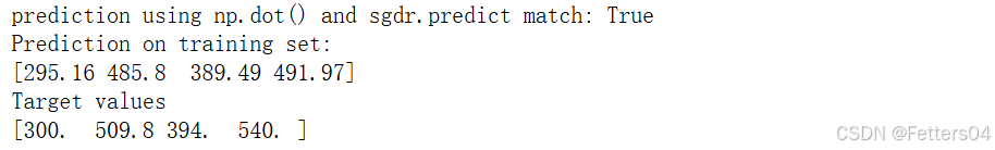
绘制预测值与目标值的关系图
py
# plot predictions and targets vs original features
fig,ax=plt.subplots(1,4,figsize=(12,3),sharey=True)
for i in range(len(ax)):
    ax[i].scatter(X_train[:,i],y_train, label = 'target')
    ax[i].set_xlabel(X_features[i])
    ax[i].scatter(X_train[:,i],y_pred,color=dlorange, label = 'predict')
ax[0].set_ylabel("Price"); ax[0].legend();
fig.suptitle("target versus prediction using z-score normalized model")
plt.show()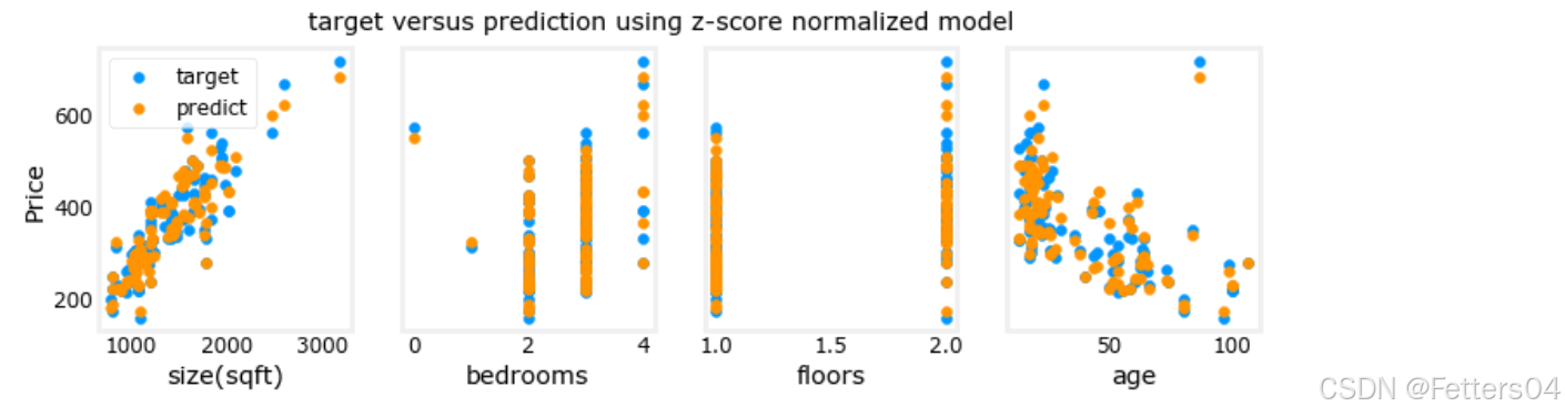
✨恭喜你,已初次使用开源机器学习包 scikit-learn ,并知道了如何使用工具包中的 梯度下降 SGDRegressor 和 特征归一化 StandardScaler 实现线性回归。