机器学习--卷积神经网络（包括python实现）

卷积神经网络

1. 计算方法

（1）输入和输出channel = 1时

首先我们要知道channel是什么意思，顾名思义channel就是"通道"的意思qwq。我们来举个例子，在计算机视觉中，如果一张图片是黑白的，那么每个像素点都是有一个信息也就是这个像素点的灰度。但是对于一张彩色图片来说，每个像素点都是由三个信息叠加而成的，也就是 R B G RBG RBG 三个颜色的"灰度"。

于是我们对黑白照片操作变成矩阵的时候，我们就会直接将灰度拿来用，把它变成一个二维的矩阵。

而对于彩色照片来说，我们就会建立一个高为 3 3 3 的三维张量来存储这个图片。这里的所谓"高度3"就是我们的channel。

这里我们先说只有一个通道的时候（也就是二维的时候）卷积网络的计算方法，我们来看这样一个图：

这里就很形象的展示了卷积的计算方法，其中 3 × 3 3 \times 3 3×3 的矩阵我们叫做 输入矩阵 ， 2 × 2 2 \times 2 2×2 的蓝色矩阵叫做 核函数 ，最后得到的 2 × 2 2 \times 2 2×2 的白色矩阵叫做 输出矩阵。

其中，我们有：

0 × 0 + 1 × 1 + 3 × 2 + 4 × 3 = 19 0 × 1 + 2 × 1 + 4 × 2 + 5 × 3 = 25 3 × 0 + 4 × 1 + 6 × 2 + 7 × 3 = 37 4 × 0 + 5 × 1 + 7 × 2 + 8 × 3 = 43 0 \times 0 + 1 \times 1 + 3 \times 2 + 4 \times 3 = 19 \\ 0 \times 1 + 2 \times 1 + 4 \times 2 + 5 \times 3 = 25 \\ 3 \times 0 + 4 \times 1 + 6 \times 2 + 7 \times 3 = 37 \\ 4 \times 0 + 5 \times 1 + 7 \times 2 + 8 \times 3 = 43 0×0+1×1+3×2+4×3=190×1+2×1+4×2+5×3=253×0+4×1+6×2+7×3=374×0+5×1+7×2+8×3=43

这就是最基本的计算方法了。

用代码写出来就是这样：

from mxnet import gluon, np, npx, autograd, nd
from mxnet.gluon import nn

data = nd.arange(9).reshape((1, 1, 3, 3))
w = nd.arange(4).reshape((1, 1, 2, 2))
out = nd.Convolution(data, w, nd.array([0]), kernel = w.shape[2:], num_filter = w.shape[0])
print("input :", data, "\n\nweight :", w, "\n\noutput :", out)

输出出来是这样：

input : 
[[[[0. 1. 2.]
   [3. 4. 5.]
   [6. 7. 8.]]]]
<NDArray 1x1x3x3 @cpu(0)> 

weight : 
[[[[0. 1.]
   [2. 3.]]]]
<NDArray 1x1x2x2 @cpu(0)> 

output : 
[[[[19. 25.]
   [37. 43.]]]]
<NDArray 1x1x2x2 @cpu(0)>

（2）对于输入的channel > 1 但 输出的channel = 1的时候

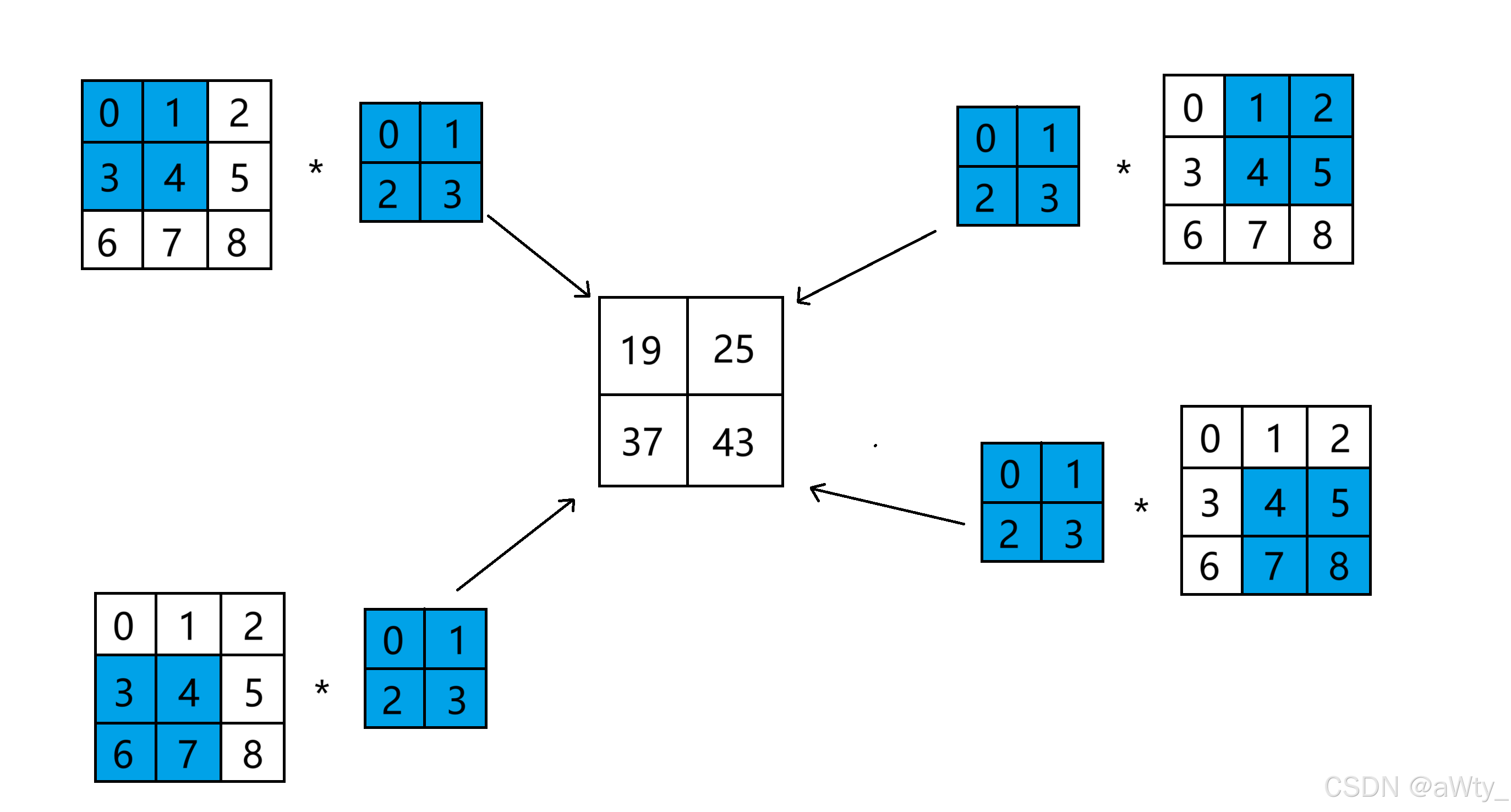
然后对于channe 输入的channel > 1但输出的channel = 1的时候，我们还是举例说明计算方法：

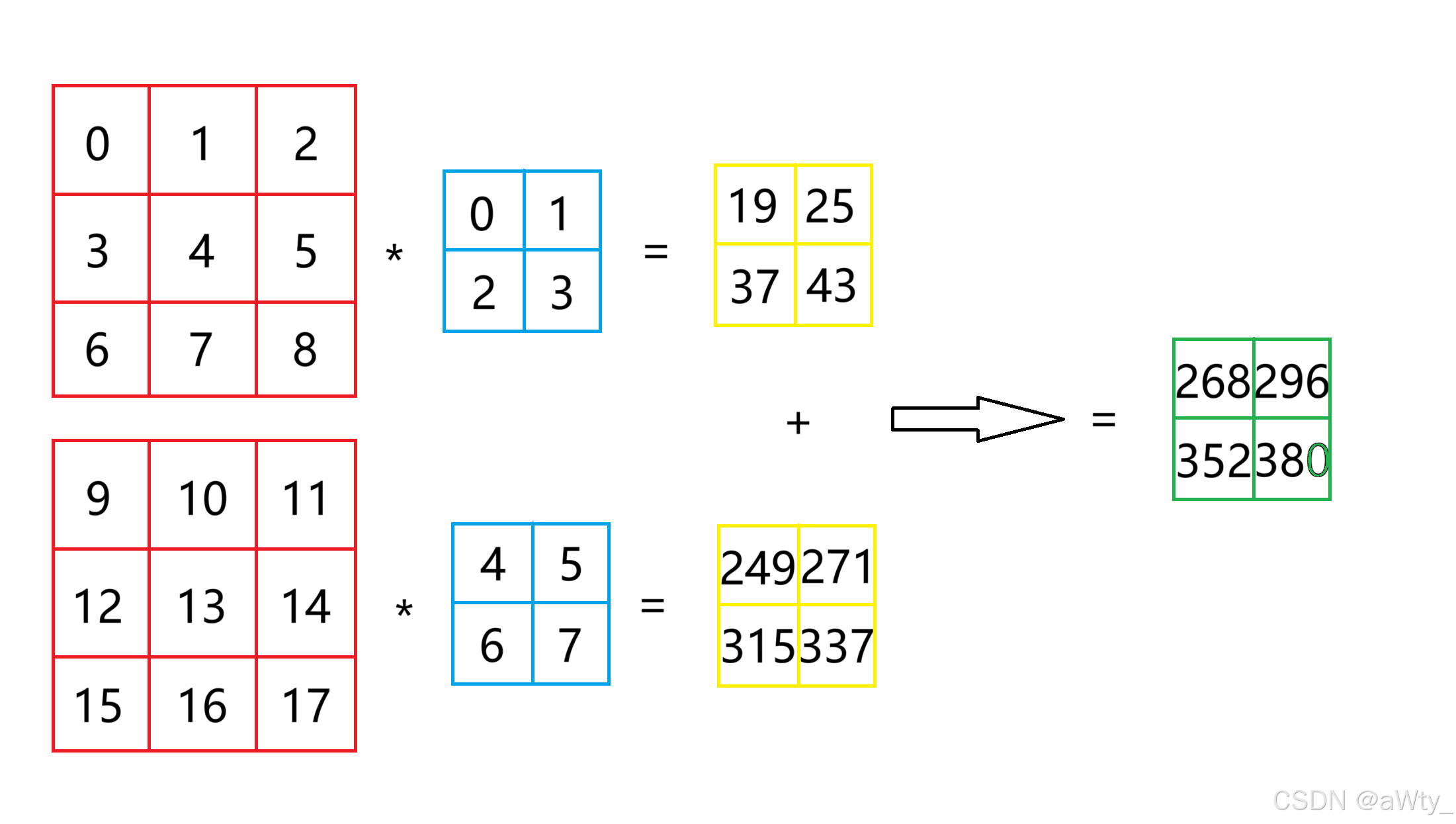
这里我们的输入矩阵变成了红色的这两个，也就是一个 2 × 3 × 3 2 \times 3 \times 3 2×3×3 的张量，而我们的核函数变成了这两个蓝色的，也就是一个 2 × 2 × 2 2 \times 2 \times 2 2×2×2 的张量。我们计算时，分别对对应的张量进行一次卷积，得到黄色的两个矩阵，然后再把这俩加起来就得到了输出矩阵。

写代码的话就是这样：

w = nd.arange(8).reshape((1, 2, 2, 2))
data = nd.arange(18).reshape((1, 2, 3, 3))
out = nd.Convolution(data, w, nd.array([0]), kernel = w.shape[2:], num_filter = w.shape[0])
print("input :", data, "\n\nweight :", w, "\n\noutput :", out)

输出就是这样：

input : 
[[[[ 0.  1.  2.]
   [ 3.  4.  5.]
   [ 6.  7.  8.]]

  [[ 9. 10. 11.]
   [12. 13. 14.]
   [15. 16. 17.]]]]
<NDArray 1x2x3x3 @cpu(0)> 

weight : 
[[[[0. 1.]
   [2. 3.]]

  [[4. 5.]
   [6. 7.]]]]
<NDArray 1x2x2x2 @cpu(0)> 

output : 
[[[[268. 296.]
   [352. 380.]]]]
<NDArray 1x1x2x2 @cpu(0)>

（3）对于输入的channel > 1 且 输出的channel > 1的时候

还是老样子，举个例子：

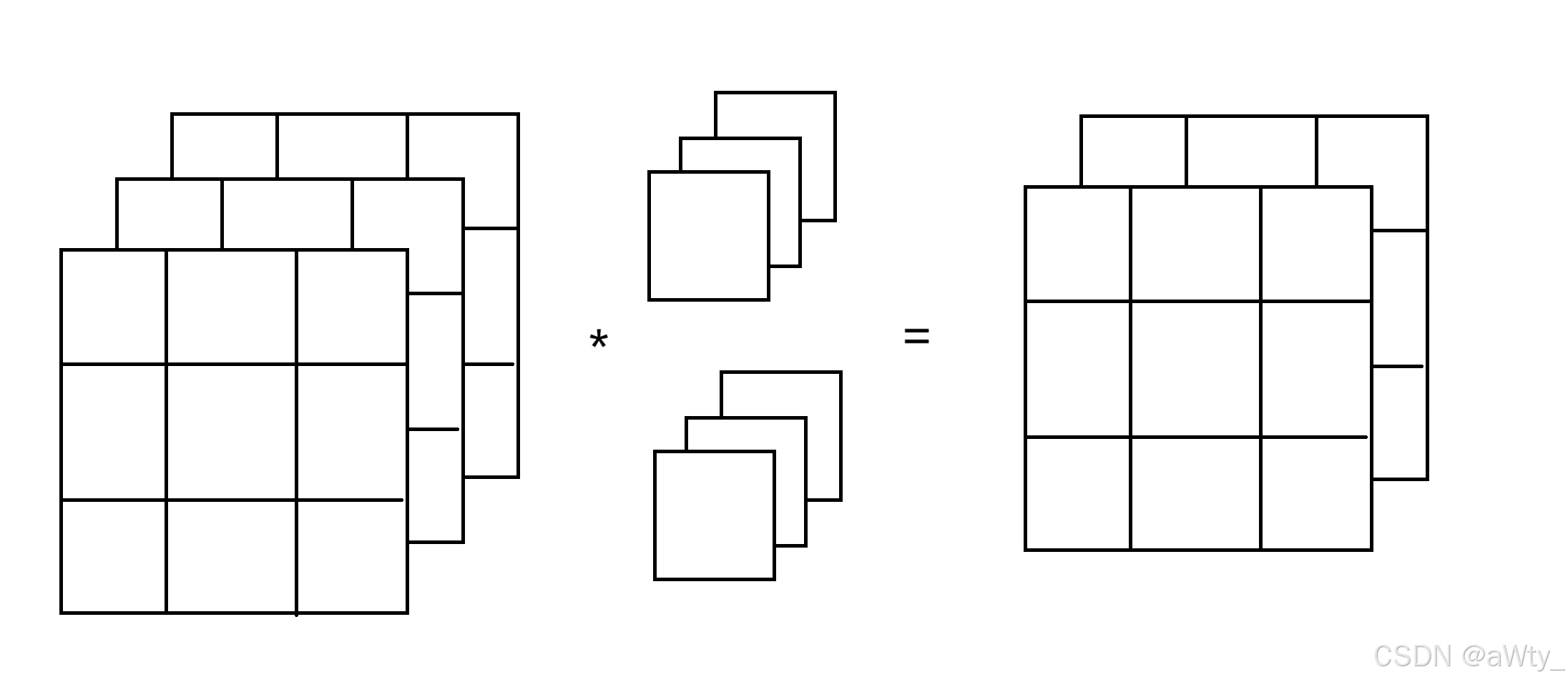
这里的输入变成了 3 × 3 × 3 3 \times 3 \times 3 3×3×3 的张量，而我们的核函数则是 2 × 3 × 1 × 1 2 \times 3 \times 1 \times 1 2×3×1×1 的张量。这里，我们的计算方法就是用核函数的第一层跟输入做一次卷积，得到第一个矩阵，然后用核函数的第二层和输入再做一次卷积得到第二个矩阵，这两个矩阵就是我们的输出了。

代码如下：

data = nd.arange(27).reshape((1, 3, 3, 3))
w = nd.arange(6).reshape((2, 3, 1, 1))
out = nd.Convolution(data, w, nd.array([0, 0]), kernel = w.shape[2:], num_filter = w.shape[0])
print("input :", data, "\n\nweight :", w, "\n\noutput :", out)

输出：

input : 
[[[[ 0.  1.  2.]
   [ 3.  4.  5.]
   [ 6.  7.  8.]]

  [[ 9. 10. 11.]
   [12. 13. 14.]
   [15. 16. 17.]]

  [[18. 19. 20.]
   [21. 22. 23.]
   [24. 25. 26.]]]]
<NDArray 1x3x3x3 @cpu(0)> 

weight : 
[[[[0.]]
  [[1.]]
  [[2.]]]

 [[[3.]]
  [[4.]]
  [[5.]]]]
<NDArray 2x3x1x1 @cpu(0)> 

output : 
[[[[ 45.  48.  51.]
   [ 54.  57.  60.]
   [ 63.  66.  69.]]

  [[126. 138. 150.]
   [162. 174. 186.]
   [198. 210. 222.]]]]
<NDArray 1x2x3x3 @cpu(0)>

（4） 关于代码的一些事

我们把刚才的三段代码贴过来，然后我们观察一下看看能不能发现什么规律：

data = nd.arange(9).reshape((1, 1, 3, 3))
w = nd.arange(4).reshape((1, 1, 2, 2))
out = nd.Convolution(data, w, nd.array([0]), kernel = w.shape[2:], num_filter = w.shape[0])
print("input :", data, "\n\nweight :", w, "\n\noutput :", out)

w = nd.arange(8).reshape((1, 2, 2, 2))
data = nd.arange(18).reshape((1, 2, 3, 3))
out = nd.Convolution(data, w, nd.array([0]), kernel = w.shape[2:], num_filter = w.shape[0])
print("input :", data, "\n\nweight :", w, "\n\noutput :", out)

data = nd.arange(27).reshape((1, 3, 3, 3))
w = nd.arange(6).reshape((2, 3, 1, 1))
out = nd.Convolution(data, w, nd.array([0, 0]), kernel = w.shape[2:], num_filter = w.shape[0])
print("input :", data, "\n\nweight :", w, "\n\noutput :", out)

我们会发现，我们的 d a t a . s h a p e data.shape data.shape 和 w . s h a p e w.shape w.shape 和 b . s h a p e b.shape b.shape 都是有讲究的，其中 d a t a . s h a p e = ( b a t c h _ s i z e , c h a n n e l s , h e i g h t , w i d t h ) data.shape = (batch\_size, channels, height, width) data.shape=(batch_size,channels,height,width)，而 w . s h a p e = ( n u m _ f i l t e r , i n p u t _ c h a n n e l s , k e r n e l _ h e i g h t , k e r n e l _ w i d t h ) w.shape = (num\_filter, input\_channels, kernel\_height, kernel\_width) w.shape=(num_filter,input_channels,kernel_height,kernel_width)。然后就是 b . s h a p e = ( 1 , n u m _ f i l t e r ) b.shape = (1, num\_filter) b.shape=(1,num_filter)

2. padding & strides

（1） 填充 Padding

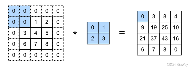
如上所述，在应用多层卷积时，我们常常丢失边缘像素。由于我们通常使用小卷积核，因此对于任何单个卷积，我们可能只会丢失几个像素。但随着我们应用许多连续卷积层，累积丢失的像素数就多了。解决这个问题的简单方法即为填充 （padding）：在输入图像的边界填充元素（通常填充元素是 0 0 0）。例如，:numref:img_conv_pad中，我们将 3 × 3 3 \times 3 3×3输入填充到 5 × 5 5 \times 5 5×5，那么它的输出就增加为 4 × 4 4 \times 4 4×4。阴影部分是第一个输出元素以及用于输出计算的输入和核张量元素： 0 × 0 + 0 × 1 + 0 × 2 + 0 × 3 = 0 0\times0+0\times1+0\times2+0\times3=0 0×0+0×1+0×2+0×3=0。

代码是这样的：

w = nd.arange(4).reshape((1, 1, 2, 2))
data = nd.arange(9).reshape((1, 1, 3, 3))
out = nd.Convolution(data, w, nd.array([0]), kernel = w.shape[2:], num_filter = w.shape[0], pad = (1, 1))       # pad:矩阵向外扩展的距离
print("input :", data, "\n\nweight :", w, "\n\noutput :", out)

output：

input : 
[[[[0. 1. 2.]
   [3. 4. 5.]
   [6. 7. 8.]]]]
<NDArray 1x1x3x3 @cpu(0)> 

weight : 
[[[[0. 1.]
   [2. 3.]]]]
<NDArray 1x1x2x2 @cpu(0)> 

output : 
[[[[ 0.  3.  8.  4.]
   [ 9. 19. 25. 10.]
   [21. 37. 43. 16.]
   [ 6.  7.  8.  0.]]]]
<NDArray 1x1x4x4 @cpu(0)>

（2） 步幅 Strides

我们看之前看到的都是每次把 k e r n e l kernel kernel 对准的一方移动一格所计算出来的输出，而 s t r i d e stride stride 就是用来控制每次移动的步幅的：

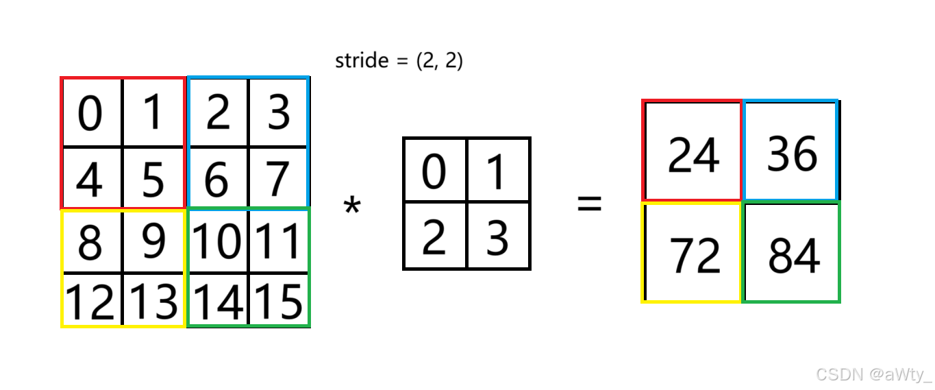
这里就是 s t r i d e = ( 2 , 2 ) stride = (2, 2) stride=(2,2) 说明步幅是 2 2 2，那我们每次移动就走两格。所以红色和 k e r n e l kernel kernel 乘起来就是 24 24 24，蓝色和 k e r n e l kernel kernel 乘起来就是 36 36 36，以此类推。

代码如下：

data = nd.arange(16).reshape((1, 1, 4, 4))
w = nd.arange(4).reshape((1, 1, 2, 2))
out = nd.Convolution(data, w, nd.array([0]), kernel = w.shape[2:], num_filter = w.shape[0], stride = (2, 2))
print("input :", data, "\n\nweight :", w, "\n\noutput :", out)

输出：

input : 
[[[[ 0.  1.  2.  3.]
   [ 4.  5.  6.  7.]
   [ 8.  9. 10. 11.]
   [12. 13. 14. 15.]]]]
<NDArray 1x1x4x4 @cpu(0)> 

weight : 
[[[[0. 1.]
   [2. 3.]]]]
<NDArray 1x1x2x2 @cpu(0)> 

output : 
[[[[24. 36.]
   [72. 84.]]]]
<NDArray 1x1x2x2 @cpu(0)>

3. 汇聚层 Pooling

与卷积层类似，汇聚层运算符由一个固定形状的窗口组成，该窗口根据其步幅大小在输入的所有区域上滑动，为固定形状窗口（有时称为汇聚窗口）遍历的每个位置计算一个输出。 然而，不同于卷积层中的输入与卷积核之间的互相关计算，汇聚层不包含参数。 相反，池运算是确定性的，我们通常计算汇聚窗口中所有元素的最大值或平均值。这些操作分别称为最大汇聚层（maximum pooling）和平均汇聚层（average pooling）

这里我们先说最大汇聚层：

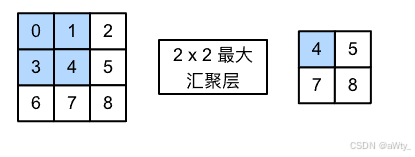
这里其实就是：

max ⁡ { 0 , 1 , 3 , 4 } = 4 max ⁡ { 1 , 2 , 4 , 5 } = 5 max ⁡ { 3 , 4 , 6 , 7 } = 7 max ⁡ { 4 , 5 , 7 , 8 } = 8 \max\{0, 1, 3, 4\} = 4 \\ \max\{1, 2, 4, 5\} = 5 \\\max\{3, 4, 6, 7\} = 7 \\ \max\{4, 5, 7, 8\} = 8 max{0,1,3,4}=4max{1,2,4,5}=5max{3,4,6,7}=7max{4,5,7,8}=8

再有就是平均汇聚层，其实跟上面一样，只是把 max ⁡ \max max 换成了 m e a n ( ) mean() mean() 而已

代码如下：

data = nd.arange(9).reshape((1, 1, 3, 3))                                                      # 关于pooling
max_pool = nd.Pooling(data = data, pool_type = 'max', kernel = (2, 2))
avg_pool = nd.Pooling(data = data, pool_type = 'avg', kernel = (2, 2))
print("data :", data, "\n\nmax pool :", max_pool, "\n\navg pool :", avg_pool)

输出：

data : 
[[[[0. 1. 2.]
   [3. 4. 5.]
   [6. 7. 8.]]]]
<NDArray 1x1x3x3 @cpu(0)> 

max pool : 
[[[[4. 5.]
   [7. 8.]]]]
<NDArray 1x1x2x2 @cpu(0)> 

avg pool : 
[[[[2. 3.]
   [5. 6.]]]]
<NDArray 1x1x2x2 @cpu(0)>

LeNet

说白了，这玩意儿就是用卷积层 convolution layer 替换了普通神经网络中的全连接层 dense layer，其他的也没什么区别...

首先就是一堆import

from mxnet import gluon
from mxnet.gluon import nn
from d2l import mxnet as d2l
from mxnet import autograd, nd
import matplotlib.pyplot as plt

然后就是定义我们的 L e N e t LeNet LeNet，也就是两层 c o n v o l u t i o n convolution convolution 每次 m a x p o o l i n g maxpooling maxpooling 一下，再搞一层 d e n s e      l a y e r dense \;\; layer denselayer 再输出：

net = nn.Sequential()
with net.name_scope():
    net.add(nn.Conv2D(channels = 20, kernel_size = 5, activation = 'relu'))
    net.add(nn.MaxPool2D(pool_size = 2, strides = 2))
    net.add(nn.Conv2D(channels = 50, kernel_size = 3, activation = 'relu'))
    net.add(nn.MaxPool2D(pool_size = 2, strides = 2))
    net.add(nn.Flatten())
    net.add(nn.Dense(128, activation = 'relu'))
    net.add(nn.Dense(10))

ctx = d2l.try_gpu()                                                  # 试试gpu能不能跑 如果报错则返回cpu
print("context :", ctx)
net.initialize(ctx = ctx)
print(net)

运行这段 代码后会输出以下内容：

context : cpu(0)
Sequential(
  (0): Conv2D(None -> 20, kernel_size=(5, 5), stride=(1, 1), Activation(relu))
  (1): MaxPool2D(size=(2, 2), stride=(2, 2), padding=(0, 0), ceil_mode=False, global_pool=False, pool_type=max, layout=NCHW)
  (2): Conv2D(None -> 50, kernel_size=(3, 3), stride=(1, 1), Activation(relu))
  (3): MaxPool2D(size=(2, 2), stride=(2, 2), padding=(0, 0), ceil_mode=False, global_pool=False, pool_type=max, layout=NCHW)
  (4): Flatten
  (5): Dense(None -> 128, Activation(relu))
  (6): Dense(None -> 10, linear)
)

然后就是从 m n i s t mnist mnist load数据下来：

batch_size, num_epoch, lr = 256, 10, 0.5
train_data, test_data = d2l.load_data_fashion_mnist(batch_size)

然后跟我们的 s o f t m a x      r e g r e s s i o n softmax \;\; regression softmaxregression 里面一样，定义一些函数：

softmax_cross_entropy = gluon.loss.SoftmaxCrossEntropyLoss()                          # 损失函数
trainer = gluon.Trainer(net.collect_params(), 'sgd', {'learning_rate' : lr})          # sgd

def accuracy(output, label):                                                          # 计算拟合的准确度
    return nd.mean(output.argmax(axis = 1) == label.astype('float32')).asscalar()     # argmax是把每一列的最大概率的index返回出来 然后和label比较是否相同 最后所有求个mean

def evaluate_accuracy(data_itetator, net, context):
    acc = 0.
    for data, label in data_itetator:
        output = net(data)
        acc += accuracy(output, label)
    return acc / len(data_itetator)

然后就是开始训练了（也和前面的 s o f t m a x      r e g r e s s i o n softmax \;\; regression softmaxregression 是一样的：

for epoch in range(num_epoch):
    train_loss, train_acc = 0., 0.
    for data, label in train_data:
        label = label.as_in_context(ctx)
        with autograd.record():
            out = net(data.as_in_context(ctx))
            loss = softmax_cross_entropy(out, label)
        loss.backward()
        trainer.step(batch_size)
        train_loss += nd.mean(loss).asscalar()
        train_acc += accuracy(out, label)
    # test_acc = 0.
    test_acc = evaluate_accuracy(test_data, net, ctx)
    print("Epoch  %d. Loss : %f, Train acc : %f, Test acc : %f" %
                (epoch, train_loss / len(train_data), train_acc / len(train_data), test_acc))

我们运行之后就能得到一下输出：

Epoch  0. Loss : 1.155733, Train acc : 0.567287, Test acc : 0.761133
Epoch  1. Loss : 0.558990, Train acc : 0.782680, Test acc : 0.826172
Epoch  2. Loss : 0.465726, Train acc : 0.821543, Test acc : 0.848633
Epoch  3. Loss : 0.420673, Train acc : 0.838697, Test acc : 0.857227
Epoch  4. Loss : 0.382026, Train acc : 0.855740, Test acc : 0.869824
Epoch  5. Loss : 0.358218, Train acc : 0.865320, Test acc : 0.871094
Epoch  6. Loss : 0.335073, Train acc : 0.873648, Test acc : 0.881641
Epoch  7. Loss : 0.317190, Train acc : 0.881250, Test acc : 0.884863
Epoch  8. Loss : 0.303633, Train acc : 0.885882, Test acc : 0.886133
Epoch  9. Loss : 0.291287, Train acc : 0.889993, Test acc : 0.886719

我们能看出这个的 t e s t      a c c u r a c y test \;\; accuracy testaccuracy 要比 s o f t m a x softmax softmax 的高很多qwq

完成代码如下：

from mxnet import gluon
from mxnet.gluon import nn
from d2l import mxnet as d2l
from mxnet import autograd, nd
import matplotlib.pyplot as plt

net = nn.Sequential()
with net.name_scope():
    net.add(nn.Conv2D(channels = 20, kernel_size = 5, activation = 'relu'))
    net.add(nn.MaxPool2D(pool_size = 2, strides = 2))
    net.add(nn.Conv2D(channels = 50, kernel_size = 3, activation = 'relu'))
    net.add(nn.MaxPool2D(pool_size = 2, strides = 2))
    net.add(nn.Flatten())
    net.add(nn.Dense(128, activation = 'relu'))
    net.add(nn.Dense(10))

ctx = d2l.try_gpu()                                                                   # 试试gpu能不能跑 如果报错则返回cpu
print("context :", ctx)
net.initialize(ctx = ctx)
print(net)

batch_size, num_epoch, lr = 256, 10, 0.5
train_data, test_data = d2l.load_data_fashion_mnist(batch_size)

softmax_cross_entropy = gluon.loss.SoftmaxCrossEntropyLoss()
trainer = gluon.Trainer(net.collect_params(), 'sgd', {'learning_rate' : lr})

def accuracy(output, label):                                                                     # 计算拟合的准确度
    return nd.mean(output.argmax(axis = 1) == label.astype('float32')).asscalar()                # argmax是把每一列的最大概率的index返回出来 然后和label比较是否相同 最后所有求个mean

def evaluate_accuracy(data_itetator, net, context):
    acc = 0.
    for data, label in data_itetator:
        output = net(data)
        acc += accuracy(output, label)
    return acc / len(data_itetator)

for epoch in range(num_epoch):
    train_loss, train_acc = 0., 0.
    for data, label in train_data:
        label = label.as_in_context(ctx)
        with autograd.record():
            out = net(data.as_in_context(ctx))
            loss = softmax_cross_entropy(out, label)
        loss.backward()
        trainer.step(batch_size)
        train_loss += nd.mean(loss).asscalar()
        train_acc += accuracy(out, label)
    # test_acc = 0.
    test_acc = evaluate_accuracy(test_data, net, ctx)
    print("Epoch  %d. Loss : %f, Train acc : %f, Test acc : %f" %
                (epoch, train_loss / len(train_data), train_acc / len(train_data), test_acc))