Numpy
创建数组
import numpy as np
创建数组
arr1=np.array(1,2,3)
arr2=np.array(\[3,4,5,2,4,1])
print(arr1)
print(arr2)
print(type(arr1))
1 2 3
\[3 4 5
2 4 1\]
<class 'numpy.ndarray'>
查看数组的基础属性
print(arr1.shape)
print(arr1.ndim)
print(arr1.dtype)
print(arr2.shape)
print(arr2.ndim)
print(arr2.dtype)
(3,)
1
int32
(2, 3)
2
int32
初识数组特点
list1=(0.3,0.5,4.2)
arr1=np.array(0.3,0.5,4.2)
print(list1)
print(arr1)
print(list1 ** 2)
print(i\*\*2 for i in list1)
print(arr1 ** 2)
0.3, 0.5, 4.2
0.3 0.5 4.2
0.09, 0.25, 17.64
0.09 0.25 17.64
创建常见数组
arr3=np.arange(0,10)
arr4=np.arange(10)
arr5=np.arange(0,1,0.1)
print(arr3)
print(arr4)
print(arr5)
0 1 2 3 4 5 6 7 8 9
0 1 2 3 4 5 6 7 8 9
0. 0.1 0.2 0.3 0.4 0.5 0.6 0.7 0.8 0.9
arr6=np.linspace(0,1,10)
print(arr6)
0. 0.1 0.2 0.3 0.4 0.5 0.6 0.7 0.8 0.9 1.
arr7=np.zeros(3,4,5)
print(arr7)
\[\[ 0. 0. 0. 0. 0.
0. 0. 0. 0. 0.
0. 0. 0. 0. 0.
0. 0. 0. 0. 0.\]
\[ 0. 0. 0. 0. 0.
0. 0. 0. 0. 0.
0. 0. 0. 0. 0.
0. 0. 0. 0. 0.\]
\[ 0. 0. 0. 0. 0.
0. 0. 0. 0. 0.
0. 0. 0. 0. 0.
0. 0. 0. 0. 0.\]\]
arr8=np.ones(3,4,5)
print(arr8)
\[\[ 1. 1. 1. 1. 1.
1. 1. 1. 1. 1.
1. 1. 1. 1. 1.
1. 1. 1. 1. 1.\]
\[ 1. 1. 1. 1. 1.
1. 1. 1. 1. 1.
1. 1. 1. 1. 1.
1. 1. 1. 1. 1.\]
\[ 1. 1. 1. 1. 1.
1. 1. 1. 1. 1.
1. 1. 1. 1. 1.
1. 1. 1. 1. 1.\]\]
数组的数据类型
arr8=np.array(3,4,5,dtype=np.float) # 声明数组的数据类型
print(arr8)
print(arr8.dtype)
arr80=1.2
print(arr8)
print(np.int32(arr8)) # 转换数组的数据类型
3. 4. 5.
float64
1.2 4. 5.
1 4 5
生成随机数
print(np.random.random(10))
[ 0.73744669 0.80080002 0.69015703 0.51743988 0.05570415 0.34901843
0.0734643 0.86541768 0.18830607 0.07036505]
print(np.random.rand(10))
[ 0.27580848 0.69278954 0.12912278 0.53180506 0.21617686 0.4357371
0.92604774 0.19278177 0.81396217 0.15550441]
print(np.random.rand(3,4))
print(np.random.randn(3,4))
\[ 0.03654586 0.23675581 0.35543946 0.31476077
0.12875907 0.78566879 0.87653987 0.78687239
0.79805071 0.46032083 0.08375826 0.60476404\]
\[ 0.22623064 -0.34199973 -0.50766523 0.01726679
0.71462127 -1.19509683 -0.3916739 0.67375221
-1.02150652 0.98995901 1.64691806 0.81784057\]
数组的索引
arr1=np.array(0.3,0.78,0.24,5,3.2)
print(arr1)
print(arr10)
print(arr1-5)
print(arr11:2)
print(arr1-4:-2)
0.3 0.78 0.24 5. 3.2
0.3
0.3
0.78
0.78 0.24
逻辑型索引
arr2=np.array(2.3,1.8,4.5)
print(arr2)
print(arr2\[False,False,True])
index=arr2>2
print(arr2index)
2.3 1.8 4.5
4.5
2.3 4.5
多维数组的索引
arr3=np.arange(1,13).reshape(3,4)
print(arr3)
print(arr32,3)
print(arr32,0:)
print(arr3:,3)
print(arr31:,1:3)
\[ 1 2 3 4
5 6 7 8
9 10 11 12\]
12
9 10 11 12
4 8 12
\[ 6 7
10 11\]
\[ 5 6 7 8
9 10 11 12\]
False True True
修改数组中的元素
arr3=np.arange(1,13).reshape(3,4)
print(arr3)
arr30,0=15
print(arr3)
\[ 1 2 3 4
5 6 7 8
9 10 11 12\]
\[15 2 3 4
5 6 7 8
9 10 11 12\]
求解距离矩阵
n=10 # 样本个数
x=np.linspace(1,100,n) # 样本的横坐标
y=np.linspace(1,100,n) # 样本的纵坐标
dist=np.sqrt((x0-x1)**2+(y0-y1)**2)
dist = np.zeros(n, n) # 初始距离矩阵
for i in range(n):
for j in range(n):
disti, j = np.sqrt((xi - xj)**2 + (yi - yj)**2) # 计算欧式距离
print(x)
print(y)
print(dist)
1. 12. 23. 34. 45. 56. 67. 78. 89. 100.
1. 12. 23. 34. 45. 56. 67. 78. 89. 100.
[[ 0. 15.55634919 31.11269837 46.66904756 62.22539674
77.78174593 93.33809512 108.8944443 124.45079349 140.00714267]
[ 15.55634919 0. 15.55634919 31.11269837 46.66904756
62.22539674 77.78174593 93.33809512 108.8944443 124.45079349]
[ 31.11269837 15.55634919 0. 15.55634919 31.11269837
46.66904756 62.22539674 77.78174593 93.33809512 108.8944443 ]
[ 46.66904756 31.11269837 15.55634919 0. 15.55634919
31.11269837 46.66904756 62.22539674 77.78174593 93.33809512]
[ 62.22539674 46.66904756 31.11269837 15.55634919 0.
15.55634919 31.11269837 46.66904756 62.22539674 77.78174593]
[ 77.78174593 62.22539674 46.66904756 31.11269837 15.55634919
- 15.55634919 31.11269837 46.66904756 62.22539674]
[ 93.33809512 77.78174593 62.22539674 46.66904756 31.11269837
15.55634919 0. 15.55634919 31.11269837 46.66904756]
[108.8944443 93.33809512 77.78174593 62.22539674 46.66904756
31.11269837 15.55634919 0. 15.55634919 31.11269837]
[124.45079349 108.8944443 93.33809512 77.78174593 62.22539674
46.66904756 31.11269837 15.55634919 0. 15.55634919]
[140.00714267 124.45079349 108.8944443 93.33809512 77.78174593
62.22539674 46.66904756 31.11269837 15.55634919 0. ]]
数组形态变化
arr4=np.arange(1,13)
print(arr4)
print(arr4.reshape(3,4))
arr5=arr4.reshape(3,4)
print(arr5.ravel()) # 数组的展平
print(arr5.flatten('F')) #数组的纵向展平
arr6=arr4.reshape(3,4)
print(np.hstack((arr5,arr6))) # 数组的横向拼接
print(np.vstack((arr5,arr6))) # 数组的纵向拼接
1 2 3 4 5 6 7 8 9 10 11 12
\[ 1 2 3 4
5 6 7 8
9 10 11 12\]
1 2 3 4 5 6 7 8 9 10 11 12
1 5 9 2 6 10 3 7 11 4 8 12
\[ 1 2 3 4 1 2 3 4
5 6 7 8 5 6 7 8
9 10 11 12 9 10 11 12\]
\[ 1 2 3 4
5 6 7 8
9 10 11 12
1 2 3 4
5 6 7 8
9 10 11 12\]
掌握 NumPy 矩阵与通用函数
import numpy as np
matr1 = np.mat("1 2 3;4 5 6;7 8 9")
print(type(matr1))
matr2 = np.matrix(\[1, 2, 3,4, 5, 6,7, 8, 9])
np.bmat('matr1 matr2; matr1, matr2')
<class 'numpy.matrix'>
matrix(\[1, 2, 3, 1, 2, 3,
4, 5, 6, 4, 5, 6,
7, 8, 9, 7, 8, 9,
1, 2, 3, 1, 2, 3,
4, 5, 6, 4, 5, 6,
7, 8, 9, 7, 8, 9])
通用函数
arr1 = np.array(0.2, 0.4, 0.6)
arr2=np.array(0.2,0.6,0.78)
list1 = 0.2, 0.4, 0.6
print(arr1+1)
print(arr1-1)
print(arr1*2)
print(arr1/2)
print(list1*2)
print(arr1+arr2)
print(arr1>0)
print(arr1<arr2)
print(np.any(arr1==0.2))
print(np.all(arr2==0.2))
1.2 1.4 1.6
-0.8 -0.6 -0.4
0.4 0.8 1.2
0.1 0.2 0.3
0.2, 0.4, 0.6, 0.2, 0.4, 0.6
0.4 1. 1.38
True True True
False True True
True
False
广播机制
arr3 = np.arange(1, 13).reshape(4, 3)
arr4 = np.array(1, 2, 3)
arr5 = np.array(\[1, 2, 3, 4])
print(arr3)
print(arr4)
print(arr5)
print(arr3+arr4)
print(arr3+arr5)
\[ 1 2 3
4 5 6
7 8 9
10 11 12\]
1 2 3
\[1
2
3
4\]
\[ 2 4 6
5 7 9
8 10 12
11 13 15\]
\[ 2 3 4
6 7 8
10 11 12
14 15 16\]
利用 NumPy 进行统计分析
import numpy as np
读写二进制文件
arr1 = np.arange(1, 13).reshape(4, 3)
arr2 = np.arange(1, 13).reshape(3, 4)
print(arr1)
print(arr2)
\[ 1 2 3
4 5 6
7 8 9
10 11 12\]
\[ 1 2 3 4
5 6 7 8
9 10 11 12\]
读写txt文件
np.savetxt('tmp/arr1.txt', arr1, delimiter=',') # 保存数据
np.loadtxt('tmp/arr1.txt', delimiter=',') # 读取数据
array(\[ 1., 2., 3.,
4., 5., 6.,
7., 8., 9.,
10., 11., 12.])
使用数组进行简单统计分析
arr3 = np.random.randint(1, 10, (3, 4))
print(arr3)
arr3.sort(axis=0)
print(arr3)
print(arr3.argsort(axis=0))
print(np.tile(arr3, 2))
print(np.repeat(arr3, 2, axis=1))
print(arr3.mean())
print(arr3.mean(axis=0))
print(arr3.max(axis=0))
print(arr3.argmax(axis=0))
\[8 6 7 3
2 9 9 4
2 5 2 3\]
\[2 5 2 3
2 6 7 3
8 9 9 4\]
\[0 0 0 0
1 1 1 1
2 2 2 2\]
\[2 5 2 3 2 5 2 3
2 6 7 3 2 6 7 3
8 9 9 4 8 9 9 4\]
\[2 2 5 5 2 2 3 3
2 2 6 6 7 7 3 3
8 8 9 9 9 9 4 4\]
5.0
4. 6.66666667 6. 3.33333333
8 9 9 4
2 2 2 2
Pandas
import pandas as pd
读取文本数据
pd.read_csv?
data_txt = pd.read_csv('data/meal_order_info.txt',sep=' ')
data_csv = pd.read_csv('data/meal_order_info.csv', encoding='gbk', header=0)
data_csv
将数据框存储为文本文件数据
data_csv.to_csv('tmp/data_csv.csv',index=None, encoding='gbk')
data_csv
读取Excel文件
data_excel = pd.read_excel('data/meal_order_detail.xlsx',sheet_name='meal_order_detail2')
data_excel
data_excel.to_excel('tmp/data_excel.xlsx', index=None, sheet_name='test1')
掌握DataFrame的常用操作
import pandas as pd
Series系列
ser1 = pd.Series(1,2,'a',index='a','b','c')
print(ser1)
ser2 = pd.Series({'a':1,2,3,'b':'1','2','3'})
print(ser2)
a 1
b 2
c a
dtype: object
a 1, 2, 3
b 1, 2, 3
dtype: object
构造数据框(DataFrame)
d=\[1.3,2.0,3,4,2,4,1,4,2,5,1.9,7,3,1,0,11]
print(d)
df = pd.DataFrame(d, index='a', 'b', 'c', 'd', columns='A', 'B', 'C', 'D')
print(df)
d={'color':'blue','green','yellow','red','white',
'object':'ball','pen','pencil','paper','mug',
'price':1.2,1.0,0.6,0.9,1.7}
frame = pd.DataFrame(d,index='a','b','c','d','e')
print(frame)
print(pd.DataFrame(index=1, 2, columns=1, 2))
print(pd.DataFrame(1, index=1, 2, columns=1, 2))
\[1.3, 2.0, 3, 4\], \[2, 4, 1, 4\], \[2, 5, 1.9, 7\], \[3, 1, 0, 11\]
A B C D
a 1.3 2.0 3.0 4
b 2.0 4.0 1.0 4
c 2.0 5.0 1.9 7
d 3.0 1.0 0.0 11
color object price
a blue ball 1.2
b green pen 1.0
c yellow pencil 0.6
d red paper 0.9
e white mug 1.7
1 2
1 NaN NaN
2 NaN NaN
1 2
1 1 1
2 1 1
数据框的常用属性
d=\[1.3,2.0,3,4,2,4,1,4,2,5,1.9,7,3,1,0,11]
df = pd.DataFrame(d, index='a', 'b', 'c', 'd', columns='A', 'B', 'C', 'D')
print(df)
print(df.values)
print(df.index)
print(df.shape)
print(df.dtypes)
A B C D
a 1.3 2.0 3.0 4
b 2.0 4.0 1.0 4
c 2.0 5.0 1.9 7
d 3.0 1.0 0.0 11
\[ 1.3 2. 3. 4.
2. 4. 1. 4.
2. 5. 1.9 7.
3. 1. 0. 11. \]
Index('a', 'b', 'c', 'd', dtype='object')
(4, 4)
A float64
B float64
C float64
D int64
dtype: object
数据框的查改增删操作
import pandas as pd
访问数据框中的元素
d=\[1.3,2.0,3,4,2,4,1,4,2,5,1.9,7,3,1,0,11]
df = pd.DataFrame(d, index='a', 'b', 'c', 'd', columns='A', 'B', 'C', 'D')
print(df)
print(df'A') # 单列数据访问
print(df\['A', 'C']) # 多列数据访问
A B C D
a 1.3 2.0 3.0 4
b 2.0 4.0 1.0 4
c 2.0 5.0 1.9 7
d 3.0 1.0 0.0 11
a 1.3
b 2.0
c 2.0
d 3.0
Name: A, dtype: float64
A C
a 1.3 3.0
b 2.0 1.0
c 2.0 1.9
d 3.0 0.0
print(df.head(3)) # 访问某几行数据
print(df.tail(3))
A B C D
a 1.3 2.0 3.0 4
b 2.0 4.0 1.0 4
c 2.0 5.0 1.9 7
A B C D
b 2.0 4.0 1.0 4
c 2.0 5.0 1.9 7
d 3.0 1.0 0.0 11
print(df)
print(df.iloc0, 0) # 按照行列顺序进行数据访问
print(df.iloc0:3, 0)
print(df.iloc:, 0)
print(df.iloc0, :)
print(df.iloc1:3, 1:3)
A B C D
a 1.3 2.0 3.0 4
b 2.0 4.0 1.0 4
c 2.0 5.0 1.9 7
d 3.0 1.0 0.0 11
1.3
a 1.3
b 2.0
c 2.0
Name: A, dtype: float64
a 1.3
b 2.0
c 2.0
d 3.0
Name: A, dtype: float64
A 1.3
B 2.0
C 3.0
D 4.0
Name: a, dtype: float64
B C
b 4.0 1.0
c 5.0 1.9
<class 'pandas.core.series.Series'>
print(df.loc'a', 'A') # 按照行列名称进行数据访问
print(df.loc'a':'c', 'A')
print(df.loc:, 'A')
print(df.loc'a', :)
print(df.loc\['b','c', 'B', 'C'])
1.3
a 1.3
b 2.0
c 2.0
Name: A, dtype: float64
a 1.3
b 2.0
c 2.0
d 3.0
Name: A, dtype: float64
A 1.3
B 2.0
C 3.0
D 4.0
Name: a, dtype: float64
B C
b 4.0 1.0
c 5.0 1.9
注意如下方式返回值的区别
print(df.iloc:, 0)
print(df.iloc:, 0:1)
print(type(df.iloc:, 0))
print(type(df.iloc:, 0:1))
a 1.3
b 2.0
c 2.0
d 3.0
Name: A, dtype: float64
A
a 1.3
b 2.0
c 2.0
d 3.0
<class 'pandas.core.series.Series'>
<class 'pandas.core.frame.DataFrame'>
修改数据框中的元素
d=\[1.3,2.0,3,4,2,4,1,4,2,5,1.9,7,3,1,0,11]
df = pd.DataFrame(d, index='a', 'b', 'c', 'd', columns='A', 'B', 'C', 'D')
print(df)
df.loc'a', 'A' = 101
df.loc:, 'B' = 0.25
df.loc:, 'C' = 1, 2, 3, 4
print(df)
A B C D
a 1.3 2.0 3.0 4
b 2.0 4.0 1.0 4
c 2.0 5.0 1.9 7
d 3.0 1.0 0.0 11
A B C D
a 101.0 0.25 1 4
b 2.0 0.25 2 4
c 2.0 0.25 3 7
d 3.0 0.25 4 11
C:\Users\Administrator\AppData\Local\Temp\ipykernel_70148\2679651701.py:7: DeprecationWarning: In a future version, `df.iloc:, i = newvals` will attempt to set the values inplace instead of always setting a new array. To retain the old behavior, use either `dfdf.columns\[i] = newvals` or, if columns are non-unique, `df.isetitem(i, newvals)`
df.loc:, 'C' = 1, 2, 3, 4
为数据框增添数据
d=\[1.3,2.0,3,4,2,4,1,4,2,5,1.9,7,3,1,0,11]
df = pd.DataFrame(d, index='a', 'b', 'c', 'd', columns='A', 'B', 'C', 'D')
print(df)
df'E' = 5
df'F' = 1, 2, 3, 4
print(df)
A B C D
a 1.3 2.0 3.0 4
b 2.0 4.0 1.0 4
c 2.0 5.0 1.9 7
d 3.0 1.0 0.0 11
A B C D E F
a 1.3 2.0 3.0 4 5 1
b 2.0 4.0 1.0 4 5 2
c 2.0 5.0 1.9 7 5 3
d 3.0 1.0 0.0 11 5 4
import pandas as pd
删除数据框中的元素
d=\[1.3,2.0,3,4,2,4,1,4,2,5,1.9,7,3,1,0,11]
df = pd.DataFrame(d, index='a', 'b', 'c', 'd', columns='A', 'B', 'C', 'D')
print(df)
print(df.drop('D'))
print(df.drop('D', axis=1, inplace=False)) # 删除数据框的列元素
print(df)
print(df.drop('a', 'c', axis=0)) # 输出数据框的行元素
A B C D
a 1.3 2.0 3.0 4
b 2.0 4.0 1.0 4
c 2.0 5.0 1.9 7
d 3.0 1.0 0.0 11
A B C
a 1.3 2.0 3.0
b 2.0 4.0 1.0
c 2.0 5.0 1.9
d 3.0 1.0 0.0
A B C D
a 1.3 2.0 3.0 4
b 2.0 4.0 1.0 4
c 2.0 5.0 1.9 7
d 3.0 1.0 0.0 11
A B C D
b 2.0 4.0 1.0 4
d 3.0 1.0 0.0 11
描述分析DataFrame数据
import numpy as np
import pandas as pd
d=\[1.3,2.0,3,4,2,4,1,4,2,5,1.9,7,3,1,0,11]
df = pd.DataFrame(d, index='a', 'b', 'c', 'd', columns='A', 'B', 'C', 'D')
print(df)
print(np.mean(df, axis=1))
print(df.mean(axis=1))
print(df.std())
print(df.describe())
print(df.T.describe())
df'A'.value_counts()
转换与处理时间序列数据
import pandas as pd
order = pd.read_csv('data/meal_order_info.csv', encoding='gbk')
print(order)
print(order'lock_time'.dtypes)
order'lock_time' = pd.to_datetime(order'lock_time')
print(order'lock_time'.dtypes)
print(pd.DatetimeIndex(order'lock_time'))
print(pd.PeriodIndex(order'lock_time', freq='H'))
order'lock_time'
print(order'lock_time'0.year) # 获取数据年份信息
print(order'lock_time'.dt.year) # 获取数据年份信息
print(order'lock_time'.dt.month) # 获取数据月份信息
print(order'lock_time'.dt.week) # 获取数据周次信息
print(order'lock_time' + pd.Timedelta(days=1)) # 时间平移
print(order'lock_time'1 - order'lock_time'0) # 求时间差别
使用分组聚合进行组内计算
import pandas as pd
detail = pd.read_excel('data/meal_order_detail.xlsx')
detail.head()
detail_group = detail\['order_id', 'counts', 'amounts'].groupby(by='order_id') # 分组操作
detail_group.agg('mean').head(3) # 对分组数据的所有列都执行mean操作
detail_group.agg('mean', 'sum').head(3) # 对分组数据的所有列都执行mean和sum操作
detail_group.agg({'counts': 'mean', np.max, 'amounts': 'std'}).head(3) # 对分组数据的不同列执行不同操作
detail_group.agg({'counts': lambda x: sum(x)**2}).head(3) # 将自定义函数放入聚合操作中
创建透视表与交叉表
import pandas as pd
detail = pd.read_excel('data/meal_order_detail.xlsx')
detail.head()
pd.pivot_table(detail\['order_id', 'counts', 'amounts'], index='order_id', aggfunc='sum').head(3)
pd.pivot_table(detail\['order_id', 'dishes_name', 'counts'], index='order_id', columns='dishes_name',aggfunc='sum').head(3)
pd.pivot_table(detail\['order_id', 'dishes_name', 'counts'], index='order_id', columns='dishes_name',values='counts', fill_value=0).head()
pd.crosstab(index=detail'order_id', columns=detail'dishes_name').head(3)
pd.crosstab(index=detail'order_id', columns=detail'dishes_name', values=detail'counts', aggfunc='sum').fillna(0).head(3)
Matplotlib
python
import numpy as np
import matplotlib.pyplot as plt
import matplotlib

x = np.arange(0, 1.1, 0.1)
print(x)
plt.figure()        # 第一环节,创建画布
plt.plot(x, x**2)   # 第二环节,绘制图形
plt.plot(x, x**4)
plt.show()          # 第三环节,显示图形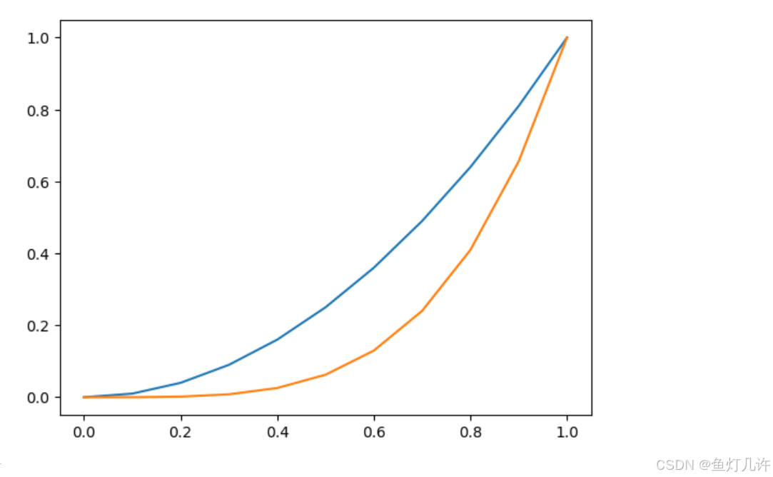
python
plt.figure

x = np.arange(0, 1.1, 0.1)
print(x)
plt.figure()        # 第一环节,创建画布
plt.plot(x, x**2)   # 第二环节,绘制图形
plt.plot(x, x**4)
plt.xlim(0, 1)
plt.ylim(0, 1)
plt.title('lines')
plt.xlabel('x')
plt.ylabel('y')
plt.legend(['y=x^2', 'y=x^4'])

plt.savefig('tmp/examplt.png')
plt.show()          # 第三环节,显示图形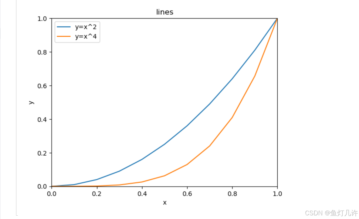
python
import numpy as np
import matplotlib.pyplot as plt

data = np.load('国民经济核算季度数据.npz', allow_pickle=True)
columns = data['columns']
values = data['values']
print(columns)
print(values)
data['values'].shape


# 绘制散点图
plt.figure(figsize=(8, 6))
plt.rcParams['font.sans-serif'] = 'SimHei'  # 设置中文显示
plt.rcParams['axes.unicode_minus'] = False

plt.scatter(values[:, 1], values[:, 3], marker='o')
plt.scatter(values[:, 1], values[:, 4], marker='*')
plt.scatter(values[:, 1], values[:, 5], marker='D')

plt.xticks(range(0, 70, 4), values[range(0, 70, 4), 1], rotation=45)
plt.legend(['第一产业生产总值', '第二产业生产总值', '第三产业生产总值'])
plt.title('2000-2017年各产业生产总值散点图')
plt.ylabel('生产总值(亿元)')
plt.savefig('tmp/2000-2017年各产业生产总值散点图.png')
plt.show()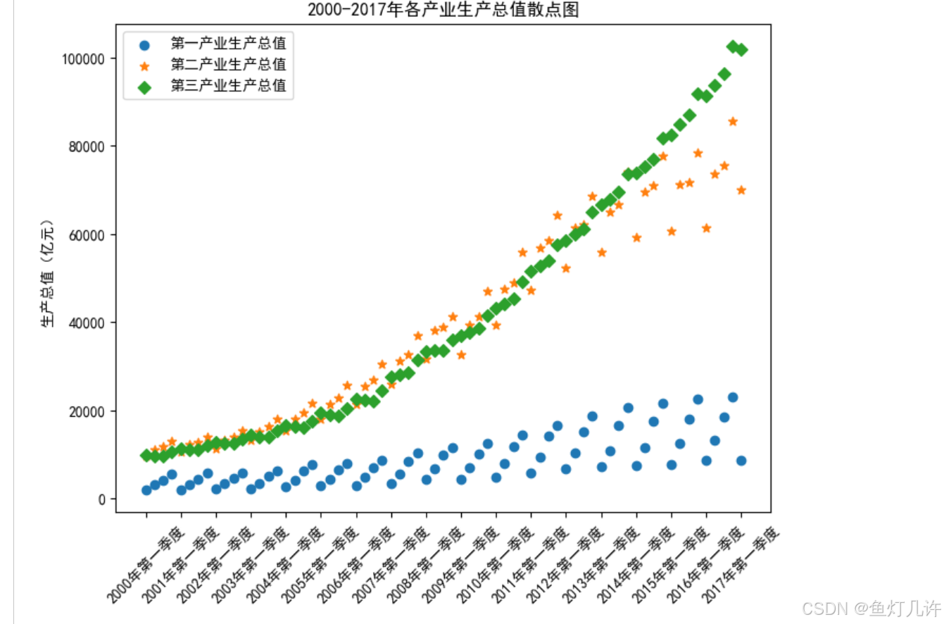
python
# 绘制折线图
plt.figure(figsize=(8, 6))
plt.rcParams['font.sans-serif'] = 'SimHei'  # 设置中文显示
plt.rcParams['axes.unicode_minus'] = False

plt.plot(values[:, 1], values[:, 3], linestyle='solid')
plt.plot(values[:, 1], values[:, 4], marker='*')
plt.plot(values[:, 1], values[:, 5], marker='D')

plt.xticks(range(0, 70, 4), values[range(0, 70, 4), 1], rotation=45)
plt.legend(['第一产业生产总值', '第二产业生产总值', '第三产业生产总值'])
plt.title('2000-2017年各产业生产总值折线图')
plt.ylabel('生产总值(亿元)')
plt.savefig('tmp/2000-2017年各产业生产总值折线图.png')
plt.show()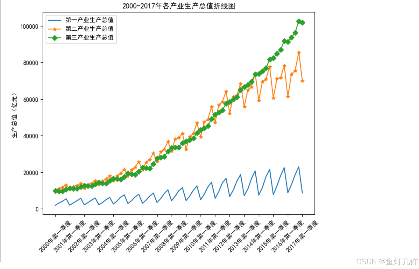
python
# 绘制直方图
plt.figure(figsize=(8, 6))
plt.rcParams['font.sans-serif'] = 'SimHei'  # 设置中文显示
plt.rcParams['axes.unicode_minus'] = False

plt.title('2017年第一季度各产业生产总值直方图')
plt.ylabel('生产总值(亿元)')
plt.bar(columns[3:6], values[-1, 3:6])
my_height = values[-1, 3:6]
for i in range(len(my_height)):
    plt.text(i, my_height[i]+1000, my_height[i], va='bottom', ha='center')

plt.show()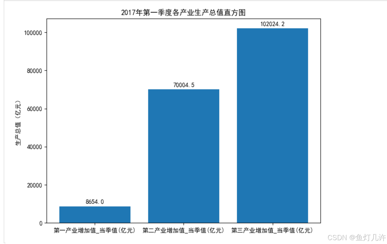
python
# 绘制饼图
plt.figure(figsize=(6, 6))
plt.rcParams['font.sans-serif'] = 'SimHei'  # 设置中文显示
plt.rcParams['axes.unicode_minus'] = False

labels = ['第一产业', '第二产业', '第三产业']

plt.pie(values[-1, 3:6], explode=[0.01, 0.01, 0.01], labels=labels, autopct='%1.1f%%')
plt.title('2017年第一季度各产业生产总值饼图')
plt.show()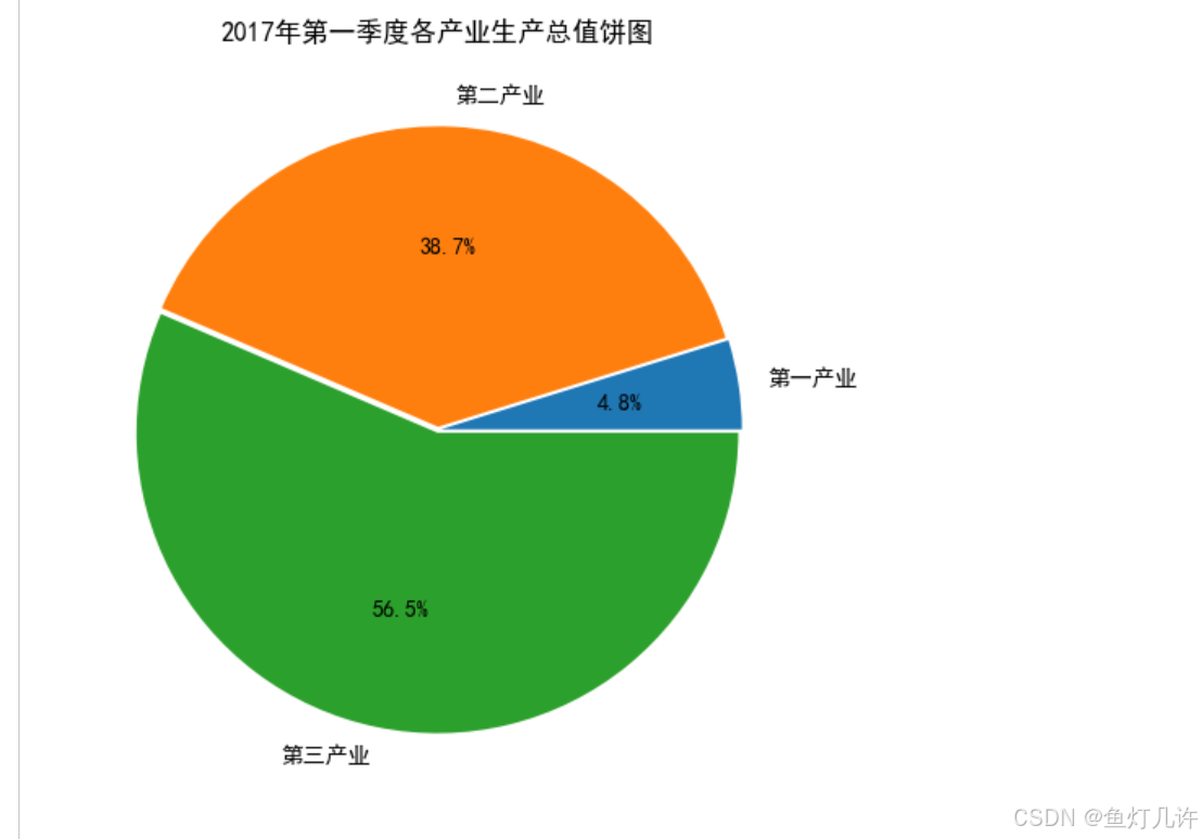
python
# 绘制箱线图
plt.figure(figsize=(6, 6))
plt.rcParams['font.sans-serif'] = 'SimHei'  # 设置中文显示
plt.rcParams['axes.unicode_minus'] = False

labels = ['第一产业', '第二产业', '第三产业']
plt.boxplot(values[:, 3:6], notch=True, labels=labels)
plt.show()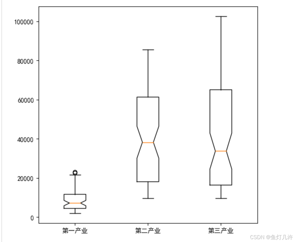
python
plt.figure(figsize=(6, 6))
plt.rcParams['font.sans-serif'] = 'SimHei'  # 设置中文显示
plt.rcParams['axes.unicode_minus'] = False

labels = ['第一产业', '第二产业', '第三产业']
plt.boxplot(values[:, 3], notch=True)
plt.show()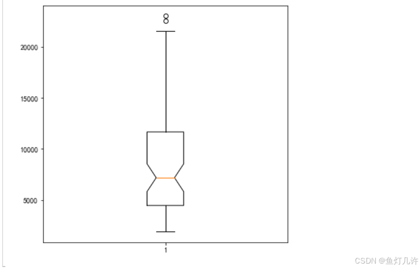
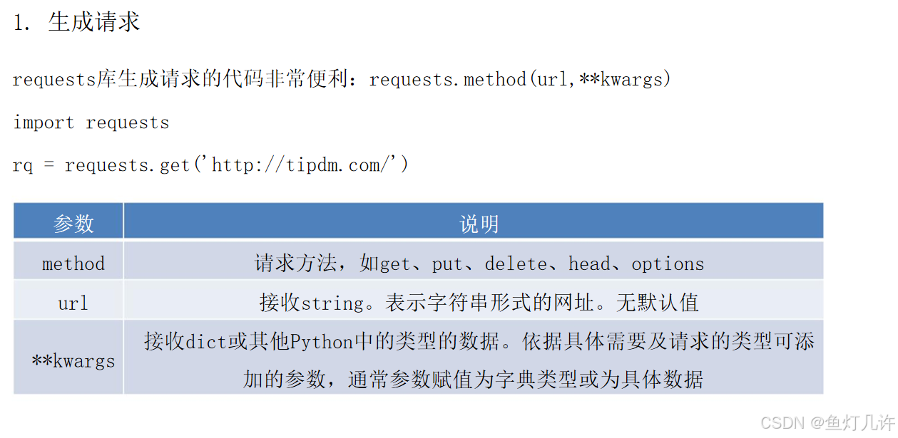
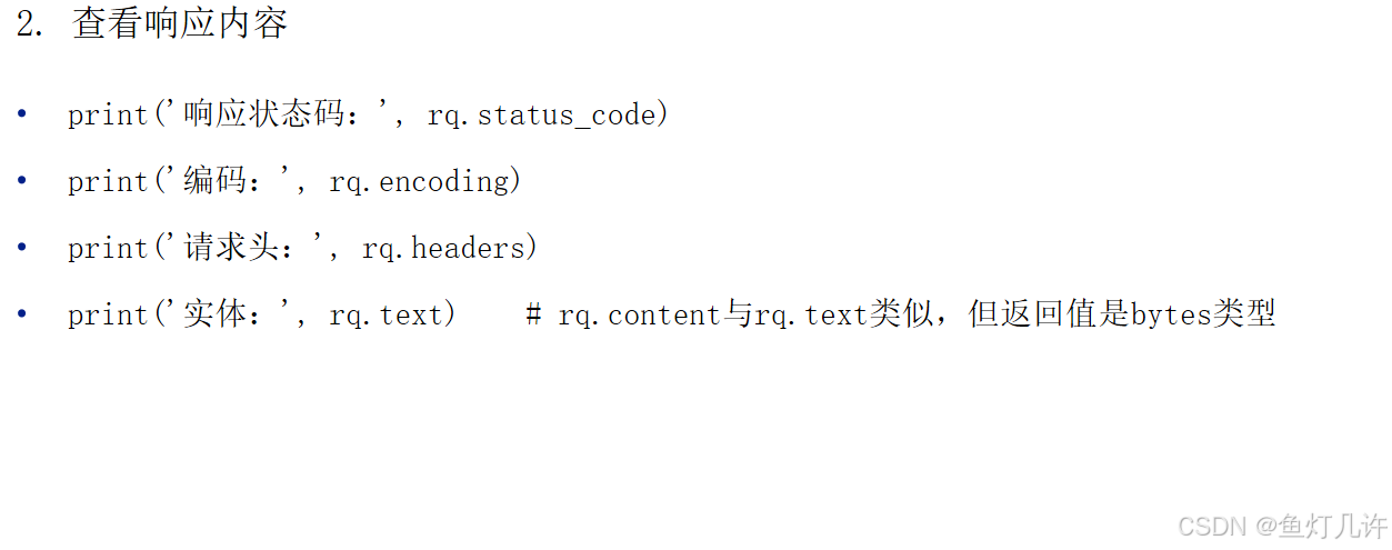
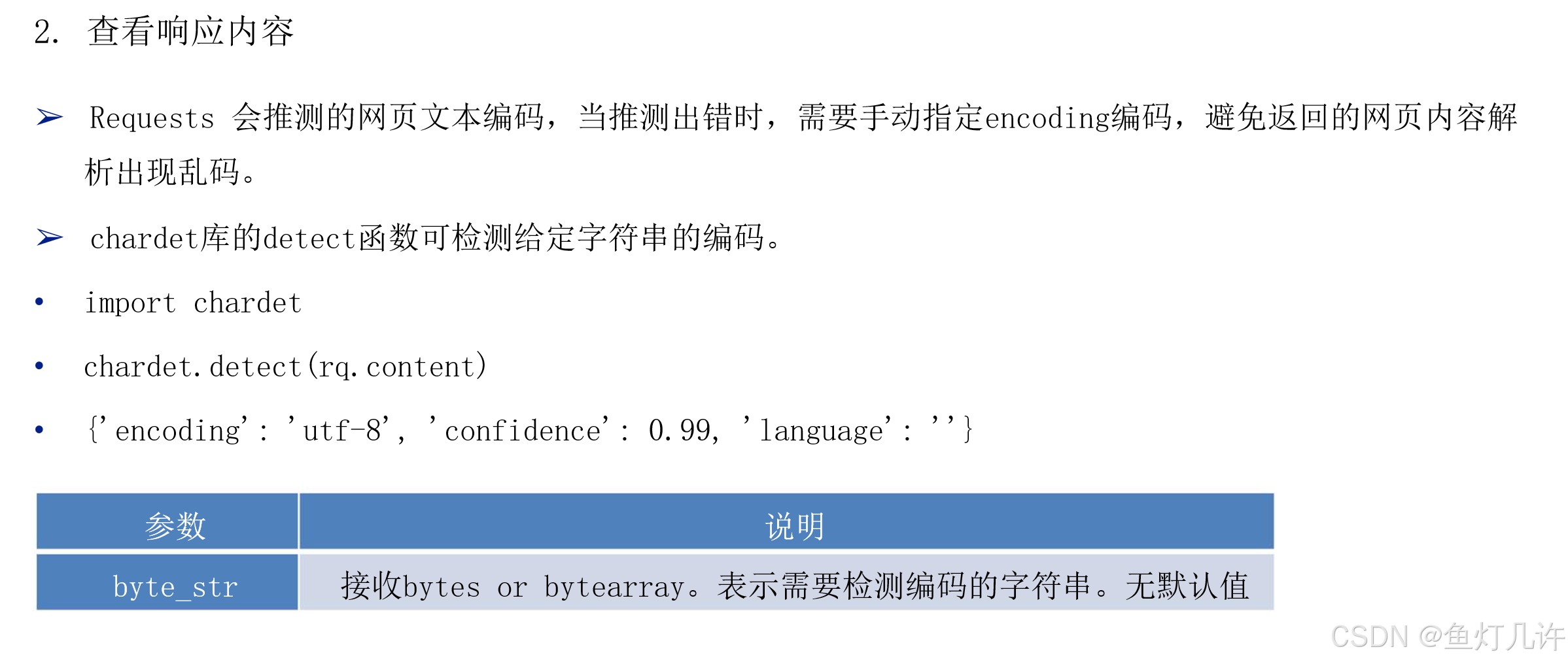
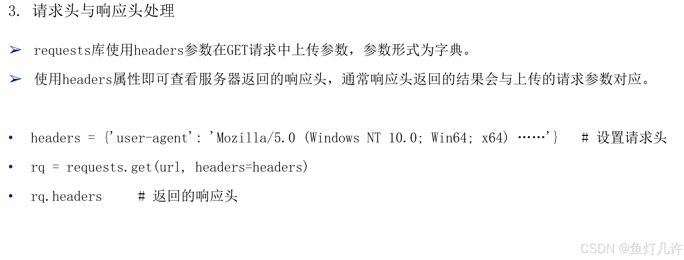
Requests库