一、人群计数的数据集包括两部分:图像部分和标签部分
1.公开数据集格式
标签部分主要包括每个人头的坐标点:(x, y);
常见的标签格式例如:ShanghaiTech数据集中的格式,用mat文件存储每个人头的坐标点,一张图像对应一个mat文件;
2.自建数据集
1)拍摄图像或者视频;视频需要切分成帧;
2)在图像上进行标点,标点的同时会记录下坐标点;
3)根据这些坐标点生成每张图像对应的.mat文件;
4)在训练时,将mat文件中的坐标转换为density map;
3.具体步骤
以下是每个步骤中所需要用到的py文件:
1)拍摄图像,如果是视频的话需要切分为视频帧:
将视频切分为视频帧:
python
import imageio

filename = "E:\video.MP4"
vid = imageio.get_reader(filename, 'ffmpeg')

try:
    for num, im in enumerate(vid):
        if (num / 50) and (num % 50) == 0:    # 控制图像的输出张数;
            imageio.imwrite('E:\save_photo_from_video\{}.jpg'.format(num // 50), im)
        else:
            continue
except imageio.core.format.CannotReadFrameError or RuntimeError:
    pass
2)在图像上进行标注:
有一些现有的工具也可以完成相应的操作,这里我们用一段py代码来实现在图像上打点并将图像上人头的坐标点写入txt文件中,已备下一步使用:
打点代码:
python
import cv2
import os

"""
This code is used to:
1)对图片进行标注
2)生成对应的包含坐标信息的.txt文件
"""

imgs_path = "E:/images/" # 存放图像的文件夹
txt_path = "E:/txt/" # 存放txt文件的文件夹
files = os.listdir(imgs_path)
img = 0
coordinates = []

def on_EVENT_LBUTTONDOWN(event, x, y, flags, param):
    if event == cv2.EVENT_LBUTTONDOWN:
        cv2.circle(img, (x, y), 4, (0, 255, 0), thickness=-1)
        coordinates.append([x, y])
        print([x,y])
        cv2.imshow("image", img)

for file in files:  # for i in range(80, len(files)):
    coordinates = []
    img = cv2.imread(imgs_path+file)
    cv2.namedWindow("image")
    cv2.setMouseCallback("image", on_EVENT_LBUTTONDOWN)
    cv2.imshow("image", img)
    cv2.waitKey(0)
    with open(txt_path+file.replace("jpg","txt"), "w+") as f:
        for coor in coordinates:
            f.write(str(coor[0])+" "+str(coor[1])+"\n")    # 记录每个人头的坐标点
        f.write(str(len(coordinates)))    # 记录一张图像中的人头总数
    print(file+" is ok !"+"\n")
使用这个打点代码时,点击运行,会出现第一张图像,然后用鼠标在上面打点,标注完一张图像后,点击右上角的×关闭这张图像,开始对第二张图像打点,直到所有图像结束;
如果中途有图像发现点错了,可以记录下错误的图像名称,待全部点完之后再进行处理;如果图像太多,一次性标注不完,建议分批进行处理;
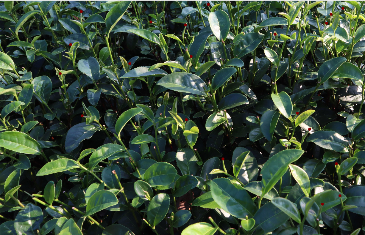
标注好图像
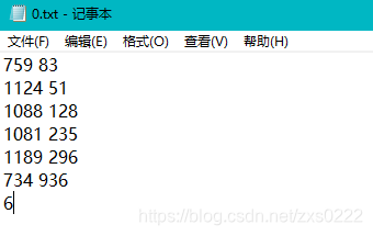
标签文件
以上就是名为0.jpg的图像打点的过程以及生成对应的0.txt,第三张图可以看到txt中的内容,为人头的坐标,最后一行为人头总数;
3)通过这些txt文件中的坐标点,形成mat文件;(注:使用ShanghaiTech数据集中的同样的格式)
将txt文件转换为mat文件:
python
import numpy as np
import scipy.io as io
import os

txt_path = "E:/txts/"
save_path = "E:/mats/"
files = os.listdir(txt_path)
for file in files:
    print(file)
    with open(txt_path+file, "r") as f:
        datas = f.readlines()
        list = []
        for i in range(0, len(datas) - 1):
            line = datas[i].strip('\n')
            ele = line.split( )
            list.append(ele)

        data_length = np.array([[datas[len(datas) - 1]]], dtype=np.uint8)

        data = np.array(list, dtype=np.float64)
        dt = np.dtype([('location', np.ndarray), ('number', np.ndarray)])
        data_combine = np.array([(data, data_length)], dtype=dt)

        image_info = np.array([data_combine], dtype=[('location', 'O'),('number', 'O')])   # [[(data, data_length)]]
        image_info = np.array([[image_info]], dtype=object)

        __header__ = b'MATLAB 5.0 MAT-file Platform: nt, Created on: 2021'
        __version__ = '1.0'
        __globals__ = '[]'

        dict = {'__header__': __header__, '__version__': __version__, '__globals__': __globals__, 'image_info':image_info}
        gt = dict["image_info"][0,0][0,0][0]

    io.savemat(save_path+file.replace("txt","mat"), dict)
通过这个步骤,我们就可以得到每张图像对应的mat文件;
4)根据mat文件制作训练时需要的density map
此处使用matlab进行实现:
a)preapre_World_10.m
matlab
clc;
clear all;

fileFolder=fullfile('F:\label');
dirOutput=dir(fullfile(fileFolder,'*'));
fileNames={dirOutput.name}';
standard_size = [384,512]; # 可以修改大小
dataset_name = ['WorldExpo10'];
original_path = ['F:/dataset/'];
output_path = 'F:/data/';
att = 'test';
train_path_img = strcat(output_path, 'train_frame/');
mkdir(train_path_img);
for ii = 3:105
  gt_path = ['F:/train_label/' fileNames{ii} '/'];

  train_path_den = strcat(output_path, 'train_lable/', fileNames{ii}, '/');
  mkdir(train_path_den);

  matFolder=fullfile(gt_path);
  matdirOutput=dir(fullfile(matFolder,'*'));
  matNames={matdirOutput.name}';
  num_images=length(matdirOutput)-1;

  disp(num_images)

  for idx = 3:num_images
    i = idx;
    if (mod(idx,10)==0)
        fprintf(1,'Processing %3d/%d files\n', idx, num_images);
    end
    load(strcat(gt_path, matNames{idx}));
    input_img_name = strcat(original_path,'train_frame/',strrep(matNames{idx}, 'mat', 'jpg'));
    disp(input_img_name)
    im = imread(input_img_name);
    [h, w, c] = size(im);
    annPoints =  point_position;

    rate_h = standard_size(1)/h;
    rate_w = standard_size(2)/w;

    im = imresize(im,[standard_size(1),standard_size(2)]);
    annPoints(:,1) = annPoints(:,1)*double(rate_w);
    annPoints(:,2) = annPoints(:,2)*double(rate_h);

    im_density = get_density_map_gaussian(im,annPoints);
    im_density = im_density(:,:,1);

    imwrite(im, [output_path 'train_frame/' strrep(matNames{idx}, 'mat', 'jpg')]);
    csvwrite([output_path 'train_lable/' fileNames{ii} '/' strrep(matNames{idx}, 'mat', 'csv')], im_density);
  end
end
b)get_density_map_gaussian()实现:
matlab
function im_density = get_density_map_gaussian(im,points)


im_density = zeros(size(im));
[h,w] = size(im_density);

if(length(points)==0)
    return;
end

if(length(points(:,1))==1)
    x1 = max(1,min(w,round(points(1,1))));
    y1 = max(1,min(h,round(points(1,2))));
    im_density(y1,x1) = 255;
    return;
end
for j = 1:length(points)
    f_sz = 15;
    sigma = 4.0;
    H = fspecial('Gaussian',[f_sz, f_sz],sigma);
    x = min(w,max(1,abs(int32(floor(points(j,1))))));
    y = min(h,max(1,abs(int32(floor(points(j,2))))));
    if(x > w || y > h)
        continue;
    end
    x1 = x - int32(floor(f_sz/2)); y1 = y - int32(floor(f_sz/2));
    x2 = x + int32(floor(f_sz/2)); y2 = y + int32(floor(f_sz/2));
    dfx1 = 0; dfy1 = 0; dfx2 = 0; dfy2 = 0;
    change_H = false;
    if(x1 < 1)
        dfx1 = abs(x1)+1;
        x1 = 1;
        change_H = true;
    end
    if(y1 < 1)
        dfy1 = abs(y1)+1;
        y1 = 1;
        change_H = true;
    end
    if(x2 > w)
        dfx2 = x2 - w;
        x2 = w;
        change_H = true;
    end
    if(y2 > h)
        dfy2 = y2 - h;
        y2 = h;
        change_H = true;
    end
    x1h = 1+dfx1; y1h = 1+dfy1; x2h = f_sz - dfx2; y2h = f_sz - dfy2;
    if (change_H == true)
        H =  fspecial('Gaussian',[double(y2h-y1h+1), double(x2h-x1h+1)],sigma);
    end
    im_density(y1:y2,x1:x2) = im_density(y1:y2,x1:x2) +  H;

end

end
4.标注完善
txt转.mat文件,这里就遇到问题了,直接用这个博客转的mat文件跟ShanghaiTech数据集是不太一样的,但因为是要往后继续生成的,它最后要生成density map,.mat只是中间文件。可以看到下图是正规ShanghaiTech数据集的GT_IMG_1.mat。
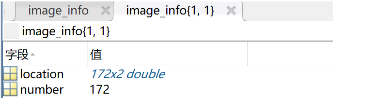
官方标注数据集
上述脚本生成的mat格式是这样子的:
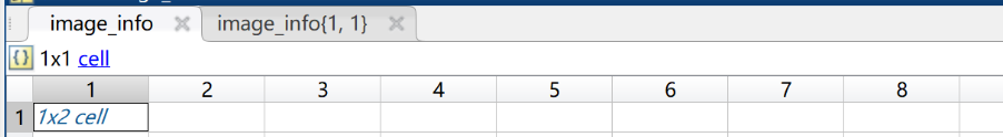
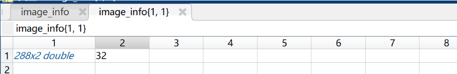
因此是不能直接使用的。不懈寻找后,可以直接用shanghaitech数据集的一个mat文件的当模板,往里套用就可以了,最后实验成功了。(ps:其实就是两块代码拼接了一下。)
代码如下:
python
from scipy.io import savemat
import numpy as np
import scipy.io as io
import os

# a = np.arange(20)
# mdic = {"a": a, "label": "experiment"}
# savemat("matlab_matrix.mat", mdic)

from scipy.io import loadmat,savemat
prototype = loadmat('F:/Scripts/crowd_counting_annotation/mats/GT_IMG_3.mat')

def convert_to_mat(prototype,dots,storeMpath):
    for i,(k,v) in enumerate(prototype.items()):
        #print(i,' Key\n',k,'\n\n',i,' Value\n',type(v))
        #print("i",i)
        #print("(k,v)",(k,v))
        #change prototypes values
        if (i==3):
            #print(111)
            #print("v",v)
            #print('v[0][0][0][0][0]',v[0][0][0][0][0])
            #make some prints first to understand on how to format your dots
            v[0][0][0][0][0] = np.array(dots,np.float64)#will replace the coordinates in the mat file
            v[0][0][0][0][1][0][0] = len(dots)#will replace an additional value of the #annotations included
            print("v[0][0][0][0][1][0][0]",v[0][0][0][0][1][0][0])
    savemat(storeMpath,prototype)


txt_path = "txt/"
save_path = "mats-1/"
files = os.listdir(txt_path)
for file in files:
    print(file)
    with open(txt_path+file, "r") as f:
        datas = f.readlines()
        print("len(datas)",len(datas))
        list = []
        for i in range(0, len(datas) - 1):
            line = datas[i].strip('\n')
            #print("line",line)
            ele = line.split( )
            #print("ele",ele)
            list.append(ele)
        #print("np.array([[datas[len(datas) - 1]]]",np.array([[datas[len(datas) - 1]]]))
        #data_length = np.array([[datas[len(datas) - 1]]], dtype=np.uint8)   #dtype=np.uint8 0~255
        #data_length = np.array([[datas[len(datas) - 1]]],dtype=int)
        #print("data_length",data_length)
        data = np.array(list, dtype=np.float64)
    storeMpath = save_path+file.replace("txt","mat")
    convert_to_mat(prototype,data,storeMpath)
**注意:**还遇到一个问题是原来的number 是dtype = uint8,但是数据会变,改成uint16就可以。也就是说模板不要用GT_IMG_1.mat,它的是uint8的,用GT_IMG_2.mat或者GT_IMG_3.mat都行。
5.补充内容
对于点的标注,可以使用Annotation Tools工具CCLabeler-master(cclabeler/CCLabeler at master · Elin24/cclabeler · GitHub),但是这块有个问题就是标注好的文件格式为JISON,里面的json文件相当于市面上数据集里的mat文件。参照ShanghaiTech数据集分成train、test,然后分成ground_truth和images子目录的结构就可以了。
具体流程如下:
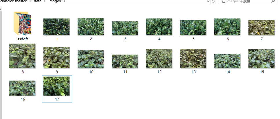
1.首先把已降低分辨率的图片都放到cclabeler-master\data\images下,并且把图片编好序号。
2.进入cclabeler-master\users\,会看到test.json文件,打开json文件,password在登录浏览器界面时要用到,data存放你待标注的图片名称(可以自己写个python脚本生成字符串),不用后缀,done和half保持空的状态。

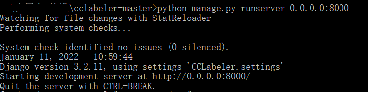
3.打开cmd,cd到cclabeler-master目录,执行python manage.py runserver 0.0.0.0:8000,出现如果提示后在浏览器输入localhost:8000再登录就OK了。
注:此处会遇到几个报错:
1)缺少模块,这个缺啥直接pip安装啥就可以。
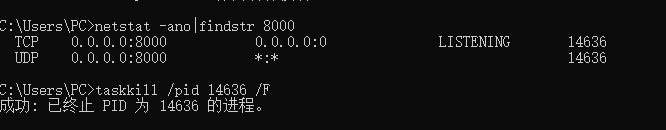
2)第二个问题报错如下:
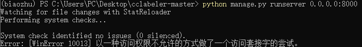
解决方案:关掉酷狗音乐的进程,因为它的串口也是:8000;另外关掉其它串口,直接cmd即可,具体指令如下:
4.界面如下,具体操作看项目的HOWTO.pdf
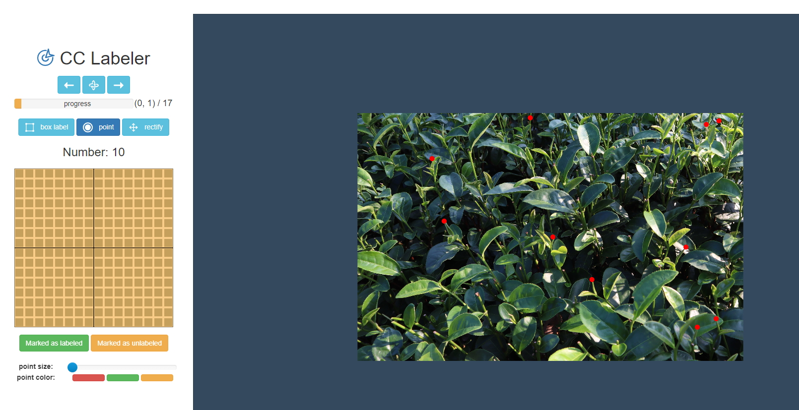
注意:此处遇到的问题:
1)点不显示的解决方案:本人最开始使用的时Chrome浏览器,无法显示点,更改为360浏览器,并对 /js/global.js文件做了如下更新:
javascript
function drawPoint(context, x, y, color = '#f00', radius = 1) {
    context.beginPath();
    context.arc(x, y, radius, 0, 2 * Math.PI);
    context.fillStyle = color;
    context.fill();
    context.closePath();
}
最终解决了标注点不显示的问题。
4.数据集整合
标注打完后,人头的位置坐标就存在cclabeler-master\data\jsons\目录下,里面的json文件相当于市面上数据集里的mat文件。参照ShanghaiTech数据集分成train、test,然后分成ground_truth和images子目录的结构就可以了。
5.DIY数据集训练
毕竟和传统数据集中mat文件不同,DIY的是json文件,所以代码相应位置也要做细微调整。只需将make_dataset.py此处更改即可,其他地方貌似没有什么要改动的,生成了GT的h5文件后,后续操作都一视同仁。
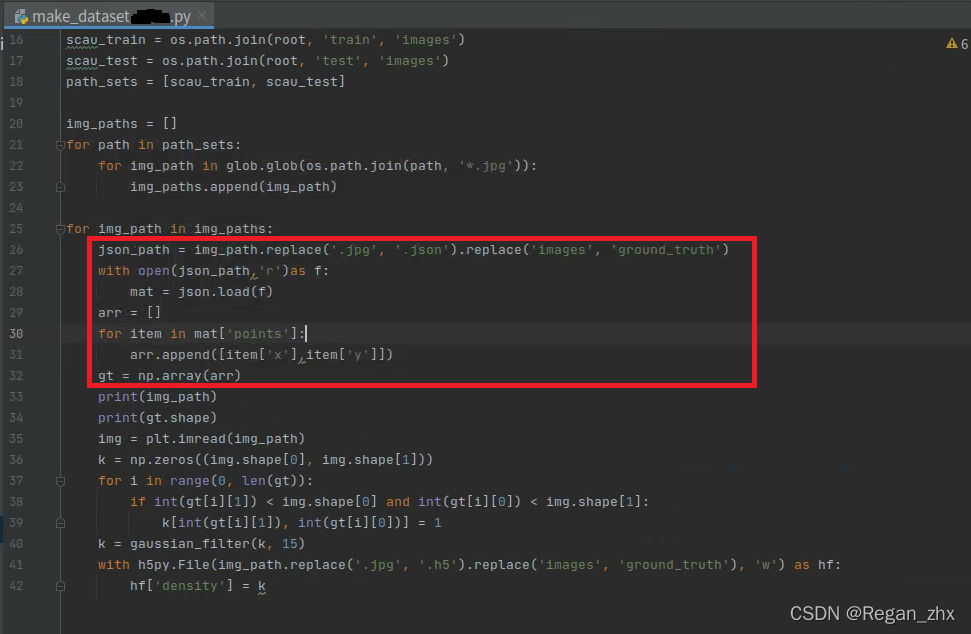
源代码自带,按照上面修改一下即可满足条件。
6.后续可视化工作补充
6.1.生成输入网络训练的密度图
如今的人群计数算法也是主流人群计数算法都是通过卷积神经网络寻找图像低级特征与密度图的映射关系,而不再是以前的图像与人数的映射关系。因此神经网络的输入就应该是密度图,输出的也应该是密度图,密度图的一大优势是可以直接积分求和,体现在python代码中就是调用sum()方法。
如下为输入网络的密度图生成代码,使用Jupyter notebook食用更佳。
python
# ipynb文件
import h5py
import scipy.io as io
import PIL.Image as Image
import numpy as np
import os
import glob
from matplotlib import pyplot as plt
from scipy.ndimage.filters import gaussian_filter
import scipy
from scipy import spatial
import json
import cv2
from matplotlib import cm as CM
from image import *
from model import CSRNet # 以CSRNet为例,此文件最好放到与项目同级目录
import torch
import random
import matplotlib.pyplot as plt
%matplotlib inline # 使用py文件请删除此行

img_path = r'SCAU_50\train\images\35.jpg' # 读者自行更改想要显示图片路径
json_path = img_path.replace('.jpg', '.json').replace('images', 'ground_truth') # 这里是自制数据集,所以读的是json文件,如果读者用已有数据集可以更改成mat文件,道理都是一样的就是读取人头位置坐标。
with open(json_path,'r')as f:
    mat = json.load(f)
arr = []
for item in mat['points']: # 由于是自制数据集是points,如果是ShanghaiTech的话可以参考项目源码对应部分
    arr.append([item['x'],item['y']])
gt = np.array(arr)
img = plt.imread(img_path)
k = np.zeros((img.shape[0], img.shape[1]))# 按图片分辨率生成零矩阵
# img.shape是先图片height然后是width,所以如下代码gt[i][1]与height比较,gt[i][0]与width比较
for i in range(0, len(gt)):
    if int(gt[i][1]) < img.shape[0] and int(gt[i][0]) < img.shape[1]:
        k[int(gt[i][1]), int(gt[i][0])] = 1  # 往零矩阵填人头坐标填1

k = gaussian_filter(k, 15)# 高斯滤波,请自行了解,这里的15是sigma值,值越大图像越模糊
plt.subplot(1,2,1) # 将plt画布分成1行2列,当前图片置于位置1
plt.imshow(img)
plt.subplot(1,2,2) # 当前图片置于位置2
plt.imshow(k,cmap=CM.jet)
plt.show()
得到如下例图:
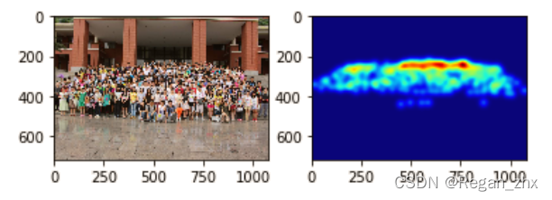
2.生成网络预测结果的密度图
在调用test.py进行预测时,神经网络读入任一张人群图片,输出一张匹配的密度图,我们接下来就显示这张密度图。
python
#ipynb文件
import sys
# 导入项目路径,这样在jupyter notebook就可以直接导入
sys.path.append(r"E:\大四上\毕设\Context-Aware-Crowd-Counting-master")
# 这里以CANNet为例,如果不是用jupyter notebook请忽略这步

import glob
from image import *
from model import CANNet
import os
import torch
from torch.autograd import Variable
from sklearn.metrics import mean_squared_error, mean_absolute_error
from torchvision import transforms
from pprint import pprint

import matplotlib.pyplot as plt
from matplotlib import cm
import matplotlib
matplotlib.rcParams['font.sans-serif'] = ['Fangsong']
matplotlib.rcParams['axes.unicode_minus'] = False
# 以上两步为设置matplotlib显示中文,这里可以忽略
%matplotlib inline

transform = transforms.Compose([
    transforms.ToTensor(), transforms.Normalize(mean=[0.485, 0.456, 0.406],
                                                std=[0.229, 0.224, 0.225]),
]) # RGB转换使用的转换器,其中的mean和std参数可以不用理会,这些数据是大家公认使用的,因为这些数值是从概率统计中得到的,直接照写即可不必深究

model = CANNet()# 导入网络模型
model = model.cuda()

checkpoint = torch.load(r'E:\Context-Aware-Crowd-Counting-master\scau_model_best.pth.tar') # 载入训练好的权重
model.load_state_dict(checkpoint['state_dict'])
model.eval() # 准备预测评估

# 指定任意一张图片即可,都是从CANNet项目源码里复制的,这里仅为作者本地所运行代码供参考
img = transform(Image.open('E:\\dataset\\SCAU_50\\train\\images\\35.jpg').convert('RGB')).cuda()
img = img.unsqueeze(0)
h, w = img.shape[2:4]
h_d = h // 2
w_d = w // 2
# 可以看出输入图片被切割成四份
img_1 = Variable(img[:, :, :h_d, :w_d].cuda())
img_2 = Variable(img[:, :, :h_d, w_d:].cuda())
img_3 = Variable(img[:, :, h_d:, :w_d].cuda())
img_4 = Variable(img[:, :, h_d:, w_d:].cuda())
density_1 = model(img_1).data.cpu().numpy()
density_2 = model(img_2).data.cpu().numpy()
density_3 = model(img_3).data.cpu().numpy()
density_4 = model(img_4).data.cpu().numpy()

# 将上部两张图片进行拼接,...为表示省略表示后面参数都全选
up_map=np.concatenate((density_1[0,0,...],density_2[0,0,...]),axis=1)
down_map=np.concatenate((density_3[0,0,...],density_4[0,0,...]),axis=1)
# 将上下部合成一张完成图片
final_map=np.concatenate((up_map,down_map),axis=0)
plt.imshow(final_map,cmap=cm.jet) # 展示图片
print(final_map.sum())# 直接输出图像预测的人数
所得示例图如下:
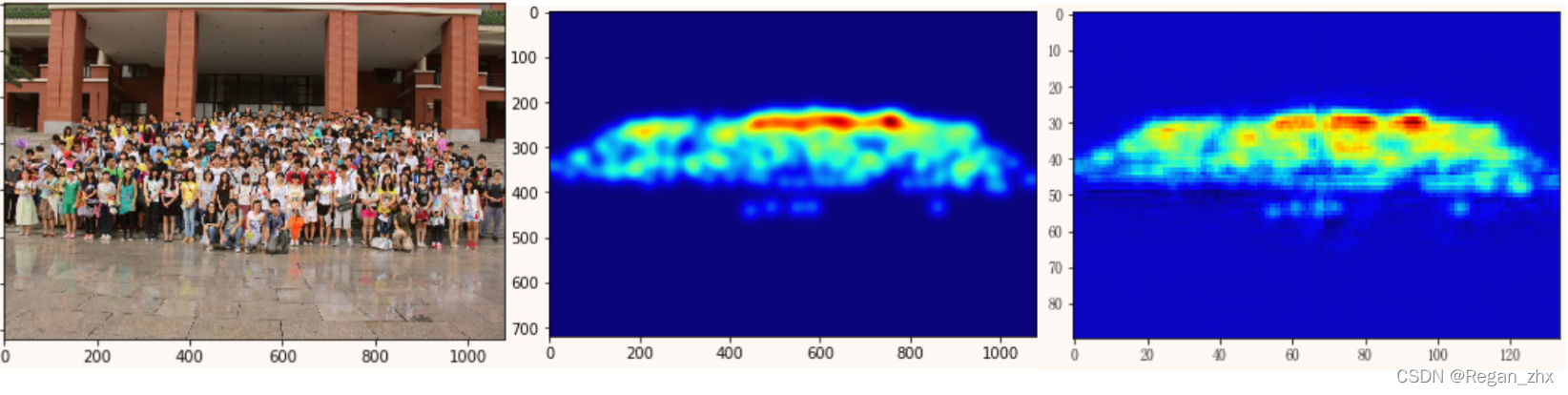
依次为原图,输入网络训练的密度图,网络预测的输出密度图。
注:主要用于个人记录使用,方便后续使用时便于查找。
参考
1、Crowdcounting用ShanghaiTech的数据集格式生成自己1730169204.html
2、https://blog.csdn.net/zxs0222/article/details/116458022
3、https://github.com/svishwa/crowdcount-mcnn/issues/33
4、cclabeler/CCLabeler at master · Elin24/cclabeler · GitHub
5、Box appears, but point does not appear · Issue #16 · Elin24/cclabeler · GitHub