从〇开始深度学习(1)——PyTorch - Python Deep Learning Neural Network API

从〇开始深度学习(1)------PyTorch - Python Deep Learning Neural Network API

文章目录

[从〇开始深度学习(1)------PyTorch - Python Deep Learning Neural Network API](#从〇开始深度学习(1)——PyTorch - Python Deep Learning Neural Network API)
- <零>写在前面
- [<壹>Part 1: Tensors and Operations](#<壹>Part 1: Tensors and Operations)
- - [1.Section 1: Introducing PyTorch](#1.Section 1: Introducing PyTorch)
  - - [1.1.PyTorch Prerequisites - Neural Network Programming Series](#1.1.PyTorch Prerequisites - Neural Network Programming Series)
    - [1.2.PyTorch Explained - Python Deep Learning Neural Network API](#1.2.PyTorch Explained - Python Deep Learning Neural Network API)
    - [1.3.PyTorch Install - Quick and Easy](#1.3.PyTorch Install - Quick and Easy)
    - [1.4.Cuda Explained - Why Deep Learning Uses GPUs](#1.4.Cuda Explained - Why Deep Learning Uses GPUs)
  - [2.Section 2: Introducing Tensors](#2.Section 2: Introducing Tensors)
  - - [2.1.Tensors Explained - Data Structures of Deep Learning](#2.1.Tensors Explained - Data Structures of Deep Learning)
    - [2.2.Rank, Axes, and Shape Explained - Tensors for Deep Learning](#2.2.Rank, Axes, and Shape Explained - Tensors for Deep Learning)
    - [2.3.CNN Tensor Shape Explained - CNNs and Feature Maps](#2.3.CNN Tensor Shape Explained - CNNs and Feature Maps)
    - [2.4.PyTorch Tensors Explained - Neural Network Programming](#2.4.PyTorch Tensors Explained - Neural Network Programming)
    - - [(1) Tensor Attributes](#(1) Tensor Attributes)
      - [(2) `torch.dtype`](#(2) torch.dtype)
      - [(3) `torch.device`](#(3) torch.device)
      - [(4) `torch.layout`](#(4) torch.layout)
      - [(5) Creating tensors using data](#(5) Creating tensors using data)
      - [(6) Creation options without data](#(6) Creation options without data)
    - [2.5.Creating PyTorch Tensors - Best Options](#2.5.Creating PyTorch Tensors - Best Options)
    - - [(1) The difference between `torch.Tensor` and `torch.tensor`](#(1) The difference between torch.Tensor and torch.tensor)
      - [(2) The difference between `torch.as_tensor` and `torch.from_numpy`](#(2) The difference between torch.as_tensor and torch.from_numpy)
      - [(3) The difference between the first two and the last two](#(3) The difference between the first two and the last two)
  - [3.Section 3: Tensor Operations](#3.Section 3: Tensor Operations)
  - - [3.1.Flatten, Reshape, and Squeeze Explained - Tensors for Deep Learning](#3.1.Flatten, Reshape, and Squeeze Explained - Tensors for Deep Learning)
    - - [(1) Reshape](#(1) Reshape)
      - [(2) Flatten](#(2) Flatten)
    - [3.2.CNN Flatten Operation Visualized - Tensor Batch Processing](#3.2.CNN Flatten Operation Visualized - Tensor Batch Processing)
    - [3.3.Tensors for Deep Learning - Broadcasting and Element-wise Operations](#3.3.Tensors for Deep Learning - Broadcasting and Element-wise Operations)
    - - [(1) Arithmetic operations](#(1) Arithmetic operations)
      - [(*) Broadcasting Tensors](#(*) Broadcasting Tensors)
      - [(2) Comparison Operations](#(2) Comparison Operations)
      - [(3) Some Functions](#(3) Some Functions)
    - [3.4.ArgMax and Reduction Ops - Tensors for Deep Learning](#3.4.ArgMax and Reduction Ops - Tensors for Deep Learning)
    - - [(1) Reduction Options](#(1) Reduction Options)
      - [(2) Argmax](#(2) Argmax)
      - [(3) Accessing elements inside tensors](#(3) Accessing elements inside tensors)
- [<贰>Part 2: Neural Network Training](#<贰>Part 2: Neural Network Training)
- - [1.Section 1: Data and Data Processing](#1.Section 1: Data and Data Processing)
  - - [1.1.Importance of Data in Deep Learning - Fashion MNIST for AI](#1.1.Importance of Data in Deep Learning - Fashion MNIST for AI)
    - [1.2.Extract, Transform, Load (ETL) - Deep Learning Data Preparation](#1.2.Extract, Transform, Load (ETL) - Deep Learning Data Preparation)
    - - [(1) What is "ETL"](#(1) What is “ETL”)
      - [(2) How to ETL with PyTorch](#(2) How to ETL with PyTorch)
    - [1.3.PyTorch Datasets and DataLoaders - Training Set Exploration](#1.3.PyTorch Datasets and DataLoaders - Training Set Exploration)
    - - [(1) PyTorch Dataset: Working with the training set](#(1) PyTorch Dataset: Working with the training set)
      - [(2) PyTorch DataLoader: Working with batches of data](#(2) PyTorch DataLoader: Working with batches of data)
      - [(3) How to Plot Images Using PyTorch DataLoader](#(3) How to Plot Images Using PyTorch DataLoader)
  - [2.Section 2: Neural Networks and PyTorch Design](#2.Section 2: Neural Networks and PyTorch Design)
  - - [2.1.Build PyTorch CNN - Object Oriented Neural Networks](#2.1.Build PyTorch CNN - Object Oriented Neural Networks)
    - - [(1) Quick object oriented programming review](#(1) Quick object oriented programming review)
      - [(2) Building a neural network in PyTorch](#(2) Building a neural network in PyTorch)
    - [2.2.CNN Layers - Deep Neural Network Architecture](#2.2.CNN Layers - Deep Neural Network Architecture)
    - - [(1) Parameter vs Argument](#(1) Parameter vs Argument)
      - [(2) Two types of parameters](#(2) Two types of parameters)
      - [(3) Descriptions of parameters](#(3) Descriptions of parameters)
      - [(4) Kernel vs Filter](#(4) Kernel vs Filter)
    - [2.3.CNN Weights - Learnable Parameters in Neural Networks](#2.3.CNN Weights - Learnable Parameters in Neural Networks)
    - - [(1) Another type of parameters](#(1) Another type of parameters)
      - [(2) Getting an Instance the Network](#(2) Getting an Instance the Network)
      - [(3) Accessing the Network's Layers](#(3) Accessing the Network's Layers)
      - [(4) Accessing the Layer Weights](#(4) Accessing the Layer Weights)
    - [2.4.Callable Neural Networks - Linear Layers in Depth](#2.4.Callable Neural Networks - Linear Layers in Depth)
    - [2.5.How to Debug PyTorch Source Code - Debugging Setup](#2.5.How to Debug PyTorch Source Code - Debugging Setup)
    - [2.6.CNN Forward Method - Deep Learning Implementation](#2.6.CNN Forward Method - Deep Learning Implementation)
    - - [(1) convolutional layers](#(1) convolutional layers)
      - [(2) linear layers](#(2) linear layers)
    - [2.7.Forward Propagation Explained - Pass Image to PyTorch Neural Network](#2.7.Forward Propagation Explained - Pass Image to PyTorch Neural Network)
    - [2.8.Neural Network Batch Processing - Pass Image Batch to PyTorch CNN](#2.8.Neural Network Batch Processing - Pass Image Batch to PyTorch CNN)
    - [2.9.CNN Output Size Formula - Bonus Neural Network Debugging Session](#2.9.CNN Output Size Formula - Bonus Neural Network Debugging Session)
  - [3.Section 3: Training Neural Networks](#3.Section 3: Training Neural Networks)
  - - [3.1.CNN Training - Using a Single Batch](#3.1.CNN Training - Using a Single Batch)
    - [3.2.CNN Training Loop - Using Multiple Epochs](#3.2.CNN Training Loop - Using Multiple Epochs)
    - [3.3.Building a Confusion Matrix - Analyzing Results Part 1](#3.3.Building a Confusion Matrix - Analyzing Results Part 1)
    - [3.4.Stack vs Concat - Deep Learning Tensor Ops](#3.4.Stack vs Concat - Deep Learning Tensor Ops)
    - [3.5.Using TensorBoard with PyTorch - Analyzing Results Part 2](#3.5.Using TensorBoard with PyTorch - Analyzing Results Part 2)
    - [3.6.Hyperparameter Experimenting - Training Neural Networks](#3.6.Hyperparameter Experimenting - Training Neural Networks)
  - [4.Section 4: Neural Network Experimentation](#4.Section 4: Neural Network Experimentation)
  - - [4.1.Custom Code - Neural Network Experimentation Code](#4.1.Custom Code - Neural Network Experimentation Code)
    - [4.2.Custom Code - Simultaneous Hyperparameter Testing](#4.2.Custom Code - Simultaneous Hyperparameter Testing)
    - [4.3.Data Loading - Deep Learning Speed Limit Increase](#4.3.Data Loading - Deep Learning Speed Limit Increase)
    - [4.4.On the GPU - Training Neural Networks with CUDA](#4.4.On the GPU - Training Neural Networks with CUDA)
    - [4.5.Data Normalization - Normalize a Dataset](#4.5.Data Normalization - Normalize a Dataset)
    - [4.6.PyTorch DataLoader Source Code - Debugging Session](#4.6.PyTorch DataLoader Source Code - Debugging Session)
    - [4.7.PyTorch Sequential Models - Neural Networks Made Easy](#4.7.PyTorch Sequential Models - Neural Networks Made Easy)
    - [4.8.Batch Norm In PyTorch - Add Normalization To Conv Net Layers](#4.8.Batch Norm In PyTorch - Add Normalization To Conv Net Layers)
- <叁>后记

<零>写在前面

有很多人学习深度学习可能会先从Python开始，然后可能会看一些吴恩达/李宏毅的课。但是我比较急性子，看Python的课很浮躁，看吴恩达/李宏毅大佬的课又很爱走神，所以我打算直接开始学习PyTorch。中间遇到Python的语法问题再去现学，等学上一段时间对深度学习有一个了解之后再回头补吴恩达/李宏毅大佬的基础课。

很难评判这种学习方法是好还是坏，毕竟我也没法做到未卜先知如果有这能力我也就不在这写学习笔记了。说一说之前的经历吧，前一阵学FPGA的时候需要现学Verilog，为了能尽快上手FPGA，我在网站上速刷了一遍Verilog基础语法就直接开始干活了（详见：什么？没有链接？总不能是隔了这么长时间还没整理笔记吧）。在实际学FPGA的时候还是遇到过因对Verilog语法不熟导致的奇怪问题，最典型的问题就是状态机的状态不能在两个always块中改变。的确，如果我一开始扎扎实实地学一遍Verilog这种脑瘫问题肯定不会应该不会吧，也不好说哈发生；但是换个角度，如果我先把这个东西用起来，用一阵有自己的理解后再回头学，会不会有不一样的效果呢？

当然了，这个操作是需要建立在掌握一门编程语言的基础上的。

回到这篇笔记，我打算把这篇笔记搞成一个完整的课程笔记，从第一节到最后一节贯穿整个系列。课程选择的是DeepLizard的PyTorch教程（相关参考链接放到后面），这套课程总共43节课，个人感觉还是不错的。不过说实话这43节的内容非常多，有一些章节都足够单拎出来写一篇笔记。所以这篇笔记还会有番外篇，如果想看完整课程笔记的话看这篇就完全OK，如果想看某些零碎的知识点可以看相应的番外篇。全系列课程分为了两个大部分，Part 1的代码非常基础，非常简单，大家有兴趣可以自己练一练；Part 2部分的代码我已经全部上传至Github和Gitee，有需要可以自行下载：

LengYuuu/PyTorchStudy_DeepLizard: This repository is used to house code for DeepLizard's PyTorch course. (github.com)

PyTorchStudy_DeepLizard: This repository is used to house code for DeepLizard's PyTorch course. (gitee.com)

这篇笔记主要是用英语写的，我的英语水平实在有限，所以想趁着看纯英课的机会涨一涨英语水平。笔记中的部分单词我也做了中文标注，如果影响到了阅读还请见谅。当然了，还是有些部分用中文写的，尤其是那些需要理解的内容，我用英语也表达不利索，如果真有人看这篇笔记的话估计也很难受，即便是我自己再回看也绝对够难受。

2024.12.05记：用英语写实在是太慢了太折磨了，TNND不练了，老老实实写中文。不过相关专业词汇还是会给出英文表达，毕竟这个实在是避不开。

笔者也是初学者，希望有问题可以和各位大佬一起交流讨论，有错误（包括英语表达的错误、语法的错误等等）还请各位指正。由于笔记篇幅过长，没有时间一一进行校对，不仅内容可能存在问题，格式也可能有没调好的地方，还请各位读者多多包容，有影响阅读的格式问题也欢迎提出。

课程链接：

PyTorch - Python Deep Learning Neural Network API - YouTube（需科学上网）

1-PyTorch Prerequisites - Syllabus for Neural Network Programming Course_哔哩哔哩_bilibili（B站搬运版，有中文字幕，非常友好）

笔记参考：

PyTorch Prerequisites - Syllabus for Neural Network Programming Course - deeplizard（需科学上网）

从零开始的机器学习实践笔记 - 知乎 (zhihu.com)（非常好的一个系列，本文提到的"知乎笔记"如无特别声明，指的就是此篇）

本文使用的环境：

环境	版本号
Windows	win11
Pycharm	2024.2.4+
Anaconda	24.11.0
Cuda	12.4.131
Python	3.10.15
PyTorch	2.5.1
torchvision	0.20.1

<壹>Part 1: Tensors and Operations

1.Section 1: Introducing PyTorch

1.1.PyTorch Prerequisites - Neural Network Programming Series

只需理解编程，不需要会很多Python。

1.2.PyTorch Explained - Python Deep Learning Neural Network API

Torch is based on the Lua programming language. PyTorch is Torch based, but in Python.

Typical packages of PyTorch:

Package	Description
torch	The top-level PyTorch package and tensor library.
torch.nn	"nn" means neural networks. A subpackage that contains classes and modules, like layers, weights and forward functions.
torch.autograd	A subpackage that handles the derivative(导数) calculations needed to optimize(优化) the neural network weights.
torch.nn.functional	A functional interface that gives us access to functions like loss functions, activation functions, and convolution(卷积) operations.
torch.optim	A subpackage that gives us access to typical optimization algorithms(算法) like SGD and Adam.
torch.utils	A subpackage that contains utility(多功能，实用) classes like datasets(数据集) and data loaders(数据加载器) that make data preprocessing much easier.
torchvision	A separate package that provides access to popular datasets, model architectures, and image transformations for computer vision.

All deep learning frameworks have two features: a tensor library, and a package for computing derivatives. And for PyTorch, these two are "torch" and "torch.autograd".
"torch.nn", "torch.autograd", "torch.nn.functional", "torch.optim", "torch.utils" are subpackages of "torch", while "torchvision" is a separate package.

Using PyTorch makes it available for us to focus more on neural networks and less on the actual framework.

The Philosophy of PyTorch:

Stay out of the way;
Cater to the impatient;
Promote linear code-flow;
Full inter-operation with the Python ecosystem;
Be as fast as anything else.

参考知乎笔记：

Another reason why we need to study PyTorch:

To optimize neural networks, we need to calculate derivatives. And to do this computationally, deep learning frameworks use what are called Computational Graphs. Computational Graphs are used to graph the function operations that occur on tensors inside neural networks. These graphs are often used to compute the derivatives needed to optimize the neural networks weights.

PyTorch uses a computational called a Dynamic(动态的) Computational Graph. This means that the graph is generated on the fly(运行中) as the operations occur. This is in contrast to static graphs that are fully determined before the actual actions occur. It just so happens that many of the cutting edge research topics in deep learning are requiring or benefiting greatly from dynamic graphs.

1.3.PyTorch Install - Quick and Easy

详见从〇开始深度学习(0)------背景知识与环境配置-CSDN博客

1.4.Cuda Explained - Why Deep Learning Uses GPUs

Much of PyTorch is written by Python, however, at bottom of points, Python drops to the C, CPP, and cuda could speed up processing and get their performance boost.

使用PyTorch不仅可以选择执行设备是CPU还是GPU，还支持多个GPU，可以选择程序在哪个GPU上执行

The calculations can be selectively carried out, either on the CPU or on the GPU.

2.Section 2: Introducing Tensors

2.1.Tensors Explained - Data Structures of Deep Learning

In Computer Science, there are: number, array, 2d-array;

In Mathematics, there are: scalar, vector, matrix;

number is same as scalar, array is same as vector, and 2d-array is same as matrix.

Indexes required	Computer science	Mathematics
0	number	scalar
1	array	vector
2	2d-array	matrix

When more than 2 indexes are required to access specific element, we stop giving specific name to the data structures, and begin using more general language.

Indexes required	Computer science	Mathematics
n	nd-array	nd-tensor

2.2.Rank, Axes, and Shape Explained - Tensors for Deep Learning

Rank：秩
- The rank of a tensor refers to the number of dimensions(维度) present within the tensor.
- A tensor's rank tells us how many indexes(索引) are needed to refer to a specific element within the tensor.
- e.g.
```
t=[
[1,2,3],
[4,5,6],
[7,8,9]
]
```
  We need two indexes to refer to a specific element, so the rank of this tensor is 2.
Axes：轴
- An axis(轴的单数形式) of a tensor is a specific dimension of a tensor.
- The rank of a tensor tells us how many axes(轴的复数形式) a tensor has.
- The length of each axis tells us how many indexes are available along each axis.
- e.g.
```
t=[
[1,2,3],
[4,5,6],
[7,8,9]
]
```
  The length of each axis is 3.
Shape：形状
- The shape of a tensor is determined by the length of each axis.
Reshape：重塑
- The shape changes the grouping of the terms but does not change the underlying(跟本的) terms themselves.
- One thing to notice about reshaping is that the product(乘积) of the component(组成部分) values in the shape must equal the total number of elements in the tensor.
- Reshaping changes the shape but not the underlying data elements.
- e.g. A 3 × 3 3×3 3×3 tensor can be reshaped to a 1 × 9 1×9 1×9 tensor.

2.3.CNN Tensor Shape Explained - CNNs and Feature Maps

The shape of a CNN input typically has a length of four. This means that we have a rank-4 tensor with four axes.

Shape: [Batch, Channels, Height, Width]

For the input tensor:
- Batch: The length of this axis tells us how many samples(样品) are in our batch.
- Channels: This axis represents the color channels. Typical values here are 3 for RGB images or 1 if we are working with grayscale(灰度) images.
- Height and Width: The image height and width. Possible values here are 28 x 28, or the 224 x 224 image size that is used by VGG16 neural network, or any other image dimensions we can imagine.
For the output tensor:
- Batch: Is same as input tensor.
- Channels: Can be seen as modified color channels.

N.B. The last axis, which is where we'll start, is where the actual numbers or data values are located.

2.4.PyTorch Tensors Explained - Neural Network Programming

When programming neural networks, data preprocessing is often one of the first steps in the overall process, and one goal of data preprocessing is to transform the raw(原始的) input data into tensor form.

(1) Tensor Attributes

Rank, Axes, and Shape is attributes for all kinds of tensor, but now we want to talk about tensors in PyTorch.

Every torch.Tensor has these attributes:torch.dtype, torch.device, and torch.layout:

torch.dtype: The dtype specifies the type of the data that is contained within the tensor.
torch.device: This determines where tensor computations for the given tensor will be performed.
torch.layout: The layout specifies how the tensor is stored in memory.

e.g.

Code:

python 复制代码

import torch

t = torch.Tensor()

print(t.dtype)
print(t.device)
print(t.layout)

Result:

torch.float32
cpu
torch.strided

(2) `torch.dtype`

Tensors contain uniform (of the same type) numerical data with one of these types:

Data type	dtype	CPU tensor	GPU tensor
32-bit floating point	torch.float32	torch.FloatTensor	torch.cuda.FloatTensor
64-bit floating point	torch.float64	torch.DoubleTensor	torch.cuda.DoubleTensor
16-bit floating point	torch.float16	torch.HalfTensor	torch.cuda.HalfTensor
8-bit integer (unsigned)	torch.uint8	torch.ByteTensor	torch.cuda.ByteTensor
8-bit integer (signed)	torch.int8	torch.CharTensor	torch.cuda.CharTensor
16-bit integer (signed)	torch.int16	torch.ShortTensor	torch.cuda.ShortTensor
32-bit integer (signed)	torch.int32	torch.IntTensor	torch.cuda.IntTensor
64-bit integer (signed)	torch.int64	torch.LongTensor	torch.cuda.LongTensor

(The table comes from PyTorch Tensors Explained - Neural Network Programming - deeplizard)

N.B. Tensor operations between tensors must happen between tensors with the same type of data.

(3) `torch.device`

PyTorch supports the use of multiple devices, and they are specified using an index like so:

python 复制代码

device = torch.device('cuda' if torch.cuda.is_available() else 'cpu')
print(device)

or:

python 复制代码

device = torch.device('cuda:0')
print(device)

The complete code is:

python 复制代码

import torch

t = torch.Tensor()

print(t.dtype)
print(t.device)
print(t.layout)

device = torch.device('cuda' if torch.cuda.is_available() else 'cpu')
print(device)
device = torch.device('cuda:0')
print(device)

And the result is:

torch.float32
cpu
torch.strided
cuda
cuda:0

So, if you have multiple GPUs, you can you can specify the GPU by different index.

N.B. Tensor operations between tensors must happen between tensors that exists on the same device.

(4) `torch.layout`

Just Don't Care.

Reference: Stride of an array - Wikipedia

(5) Creating tensors using data

python 复制代码

import torch
import numpy as np
data = np.array([1,2,3])

o1 = torch.Tensor(data)
o2 = torch.tensor(data)
o3 = torch.as_tensor(data)
o4 = torch.from_numpy(data)

print(o1)
print(o2)
print(o3)
print(o4)

The result is:

tensor([1., 2., 3.])
tensor([1, 2, 3])
tensor([1, 2, 3])
tensor([1, 2, 3])

The first option (o1) has dots after the number indicating that the numbers are floats, while the next three options have a type of int32.

(6) Creation options without data

python 复制代码

import torch
import numpy as np
data = np.array([1,2,3])

o1 = torch.eye(2)
o2 = torch.zeros([2,2])
o3 = torch.ones([2,2])
o4 = torch.rand([2,2])

print(o1)
print(o2)
print(o3)
print(o4)

The result is:

tensor([[1., 0.],
        [0., 1.]])
tensor([[0., 0.],
        [0., 0.]])
tensor([[1., 1.],
        [1., 1.]])
tensor([[0.4056, 0.8623],
        [0.5164, 0.9960]])

2.5.Creating PyTorch Tensors - Best Options

(1) The difference between `torch.Tensor` and `torch.tensor`

A quick recap:

python 复制代码

import torch
import numpy as np
data = np.array([1,2,3])

o1 = torch.Tensor(data)
o2 = torch.tensor(data)

print(o1)
print(o2)

The result is:

tensor([1., 2., 3.])
tensor([1, 2, 3])
tensor([1, 2, 3])
tensor([1, 2, 3])

The first option with the uppercase T is the constructor of the torch.Tensor class, and the second option is what we call a factory function that constructs torch.Tensor objects and returns them to the caller. (Factory functions are a software design pattern for creating objects.)

It's fine to use either one. However, the factory function torch.tensor() has better documentation and more configuration options, so it gets the winning spot at the moment.

(2) The difference between `torch.as_tensor` and `torch.from_numpy`

python 复制代码

o3 = torch.as_tensor(data)
o4 = torch.from_numpy(data)

print(o3)
print(o4)

The result is:

tensor([1, 2, 3])
tensor([1, 2, 3])

The third and the fourth option are factory functions, too.

The torch.from_numpy() function only accepts numpy.ndarrays, while the torch.as_tensor() function accepts a wide variety of array-like objects including other PyTorch tensors. For this reason, torch.as_tensor() is the winning choice.

(3) The difference between the first two and the last two

If we change the data like this:

python 复制代码

import torch
import numpy as np
data = np.array([1,2,3])

o1 = torch.Tensor(data)
o2 = torch.tensor(data)
o3 = torch.as_tensor(data)
o4 = torch.from_numpy(data)

print(o1)
print(o2)
print(o3)
print(o4)

data[0] = 0
data[1] = 0
data[2] = 0

print(o1)
print(o2)
print(o3)
print(o4)

The result is:

tensor([1., 2., 3.])
tensor([1, 2, 3])
tensor([1, 2, 3])
tensor([1, 2, 3])
tensor([1., 2., 3.])
tensor([1, 2, 3])
tensor([0, 0, 0])
tensor([0, 0, 0])

This happens because torch.Tensor() and torch.tensor() copy their input data while torch.as_tensor() and torch.from_numpy() share their input data in memory with the original input object.

Given all of these details, these two are the best options:

torch.tensor()
torch.as_tensor()

The torch.tensor() call is the sort of go-to call, while torch.as_tensor() should be employed when tuning our code for performance.

N.B.

Since numpy.ndarray objects are allocated on the CPU, the as_tensor() function must copy the data from the CPU to the GPU when a GPU is being used.
The memory sharing of as_tensor() doesn't work with built-in Python data structures like lists.
The as_tensor() call requires developer knowledge of the sharing feature. This is necessary so we don't inadvertently make an unwanted change in the underlying data without realizing the change impacts multiple objects.
The as_tensor() performance improvement will be greater if there are a lot of back and forth operations between numpy.ndarray objects and tensor objects. However, if there is just a single load operation, there shouldn't be much impact from a performance perspective.

3.Section 3: Tensor Operations

We have the following high-level categories of operations:

Reshaping operations
Element-wise operations
Reduction operations
Access operations

3.1.Flatten, Reshape, and Squeeze Explained - Tensors for Deep Learning

(1) Reshape

Code:

python 复制代码

import torch

t = torch.tensor([
    [1,1,1,1],
    [2,2,2,2],
    [3,3,3,3]
], dtype=torch.float32)
print(t)
print(t.shape)

print(t.reshape([1,12]))

print(t.reshape([2,6]))

print(t.reshape([3,4]))

print(t.reshape([4,3]))

Result:

tensor([[1., 1., 1., 1.],
        [2., 2., 2., 2.],
        [3., 3., 3., 3.]])
torch.Size([3, 4])
tensor([[1., 1., 1., 1., 2., 2., 2., 2., 3., 3., 3., 3.]])
tensor([[1., 1., 1., 1., 2., 2.],
        [2., 2., 3., 3., 3., 3.]])
tensor([[1., 1., 1., 1.],
        [2., 2., 2., 2.],
        [3., 3., 3., 3.]])
tensor([[1., 1., 1.],
        [1., 2., 2.],
        [2., 2., 3.],
        [3., 3., 3.]])

N.B. t.reshape doesn't change t itself.

Code:

python 复制代码

print(t)

Result:

tensor([[1., 1., 1., 1.],
        [2., 2., 2., 2.],
        [3., 3., 3., 3.]])

We can also increase or decrease the rank. For example:

Code:

python 复制代码

print(t.reshape([2,2,3]))

Result:

tensor([[[1., 1., 1.],
         [1., 2., 2.]],

        [[2., 2., 3.],
         [3., 3., 3.]]])

(2) Flatten

A flatten operation on a tensor reshapes the tensor to have a shape that is equal to the number of elements contained in the tensor. This is the same thing as a 1d-array of elements.

Flattening a tensor means to remove all of the dimensions except for one.

We'll see that flatten operations are required when passing an output tensor from a convolutional layer to a linear layer.

Create a Python function:

python 复制代码

def flatten(t):
    t = t.reshape(1, -1)
    t = t.squeeze()
    return t

In PyTorch, the -1 tells the reshape() function to figure out what the value should be based on the number of elements contained within the tensor.

Squeezing a tensor removes the dimensions or axes that have a length of one.

Code:

python 复制代码

print(flatten(t))

Result:

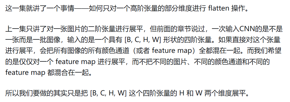
tensor([1., 1., 1., 1., 2., 2., 2., 2., 3., 3., 3., 3.])

3.2.CNN Flatten Operation Visualized - Tensor Batch Processing

In past posts, we learned about flattening an entire tensor image. But when working with CNNs, we want to only flatten specific axes within the tensor.

参考知乎笔记：

e.g.

python 复制代码

import torch

t1 = torch.tensor([
    [1,1,1,1],
    [1,1,1,1],
    [1,1,1,1],
    [1,1,1,1]
])

t2 = torch.tensor([
    [2,2,2,2],
    [2,2,2,2],
    [2,2,2,2],
    [2,2,2,2]
])

t3 = torch.tensor([
    [3,3,3,3],
    [3,3,3,3],
    [3,3,3,3],
    [3,3,3,3]
])

t = torch.stack((t1, t2, t3))
t = t.reshape(3,1,4,4)

print(t)

print(t.flatten(start_dim=1))

tensor([[[[1, 1, 1, 1],
          [1, 1, 1, 1],
          [1, 1, 1, 1],
          [1, 1, 1, 1]]],


        [[[2, 2, 2, 2],
          [2, 2, 2, 2],
          [2, 2, 2, 2],
          [2, 2, 2, 2]]],


        [[[3, 3, 3, 3],
          [3, 3, 3, 3],
          [3, 3, 3, 3],
          [3, 3, 3, 3]]]])
tensor([[1, 1, 1, 1, 1, 1, 1, 1, 1, 1, 1, 1, 1, 1, 1, 1],
        [2, 2, 2, 2, 2, 2, 2, 2, 2, 2, 2, 2, 2, 2, 2, 2],
        [3, 3, 3, 3, 3, 3, 3, 3, 3, 3, 3, 3, 3, 3, 3, 3]])

Notice in the call how we specified the start_dim parameter. This tells the flatten() method which axis it should start the flatten operation. The start_dim=1 here is an index, so it's the second axis which is the color channel axis. We skip over the batch axis so to speak, leaving it intact(完好无损的).

视频最后还留了一个思考题，如果是RGB图片想保留Color Channels应该怎么展平。把start_dim=1改为start_dim=2即可。

3.3.Tensors for Deep Learning - Broadcasting and Element-wise Operations

An element-wise operation operates on corresponding(相应的) elements between tensors.

Two elements are said to be corresponding if the two elements occupy the same position within the tensor. The position is determined by the indexes used to locate each element.

N.B. Two tensors must have the same shape in order to perform element-wise operations on them.

(1) Arithmetic operations

Arithmetic operations are element-wise operations.

Code:

python 复制代码

import torch

t1 = torch.tensor([
    [1,2],
    [3,4]
], dtype=torch.float32)

t2 = torch.tensor([
    [5,6],
    [7,8]
], dtype=torch.float32)

print(t1+t2)
print(t1-t2)
print(t1*t2)
print(t1/t2)

print(t1+3)
print(t1-3)
print(t1*3)
print(t1/3)

print(t1.add(3))
print(t1.sub(3))
print(t1.mul(3))
print(t1.div(3))

Result:

tensor([[ 6.,  8.],
        [10., 12.]])
tensor([[-4., -4.],
        [-4., -4.]])
tensor([[ 5., 12.],
        [21., 32.]])
tensor([[0.2000, 0.3333],
        [0.4286, 0.5000]])
        
tensor([[4., 5.],
        [6., 7.]])
tensor([[-2., -1.],
        [ 0.,  1.]])
tensor([[ 3.,  6.],
        [ 9., 12.]])
tensor([[0.3333, 0.6667],
        [1.0000, 1.3333]])
        
tensor([[4., 5.],
        [6., 7.]])
tensor([[-2., -1.],
        [ 0.,  1.]])
tensor([[ 3.,  6.],
        [ 9., 12.]])
tensor([[0.3333, 0.6667],
        [1.0000, 1.3333]])

(*) Broadcasting Tensors

Broadcasting is not a so called "option". But we need to know.

Broadcasting describes how tensors with different shapes are treated during element-wise operations. It is the concept whose implementation allows us to add scalars to higher dimensional tensors.

Code:

python 复制代码

import torch
import numpy as np

t1 = torch.tensor([
    [1,2],
    [3,4]
], dtype=torch.float32)

print(np.broadcast_to(3, t1.shape))

Result:

[[3 3]
 [3 3]]

This is all under the hood.

(hood: （衣服上的）兜帽，风帽；头巾，面罩；（设备或机器的）防护罩，罩；汽车发动机罩；)

(under the hood: 在表面之下：指在某物的内部工作过程中)

So, t1 + 3 is really this:

python 复制代码

t1 + torch.tensor(
    np.broadcast_to(3, t1.shape)
    ,dtype=torch.float32
)

(2) Comparison Operations

Testing code:

python 复制代码

import torch

print(torch.tensor([1, 2, 3]) < torch.tensor([3, 1, 2]))

Result:

tensor([ True, False, False])

Comparison operations are element-wise operations.

Code:

python 复制代码

import torch

t = torch.tensor([
    [0,-5,0],
    [6,0,7],
    [0,8,0]
], dtype=torch.float32)

print(t.eq(0))          # equal to
print(t.ge(0))          # greater than or equal to
print(t.gt(0))          # greater than
print(t.lt(0))          # less than
print(t.le(7))          # less than or equal to

Result:

tensor([[ True, False,  True],
        [False,  True, False],
        [ True, False,  True]])
tensor([[ True, False,  True],
        [ True,  True,  True],
        [ True,  True,  True]])
tensor([[False, False, False],
        [ True, False,  True],
        [False,  True, False]])
tensor([[False,  True, False],
        [False, False, False],
        [False, False, False]])
tensor([[ True,  True,  True],
        [ True,  True,  True],
        [ True, False,  True]])

(3) Some Functions

Code:

python 复制代码

import torch

t = torch.tensor([
    [0,-5,0],
    [6,0,7],
    [0,8,0]
], dtype=torch.float32)

print(t.abs())
print(t.sqrt())
print(t.neg())
print(t.neg().abs())

Result:

tensor([[0., 5., 0.],
        [6., 0., 7.],
        [0., 8., 0.]])
tensor([[0.0000,    nan, 0.0000],
        [2.4495, 0.0000, 2.6458],
        [0.0000, 2.8284, 0.0000]])
tensor([[-0.,  5., -0.],
        [-6., -0., -7.],
        [-0., -8., -0.]])
tensor([[0., 5., 0.],
        [6., 0., 7.],
        [0., 8., 0.]])

3.4.ArgMax and Reduction Ops - Tensors for Deep Learning

(1) Reduction Options

e.g.

Code:

python 复制代码

import torch

t = torch.tensor([
    [0,1,0],
    [2,0,2],
    [0,3,0]
], dtype=torch.float32)

print(t.sum())
print(t.prod())             # product
print(t.mean())             # average
print(t.std())              # standard deviation(标准差)

Result:

tensor(8.)
tensor(0.)
tensor(0.8889)
tensor(1.1667)

Here is a question though: Do reduction operations always reduce to a tensor with a single element?

The answer is no!

In fact, we often reduce specific axes at a time. This process is important. It's just like we saw with reshaping when we aimed to flatten the image tensors within a batch while still maintaining the batch axis.

e.g.

Code:

python 复制代码

import torch

t = torch.tensor([
    [1,1,1,1],
    [2,2,2,2],
    [3,3,3,3]
], dtype=torch.float32)

print(t.sum(dim=0))
print(t.sum(dim=1))

Result:

tensor([6., 6., 6., 6.])
tensor([ 4.,  8., 12.])

回顾这句话：reduce specific axes at a time。

如何表示张量t里的某一元素？t[dim0][dim1]。

dim	dim1=0	dim1=1	dim1=2	dim1=3
dim0=0	1	1	1	1
dim0=1	2	2	2	2
dim0=2	3	3	3	3

减少dim0，求和操作会纵向相加；减少dim1，求和操作会横向相加。其实第二个结果如果写成这样会更好理解：

tensor([ 	4.,
			8.,
            12.		])

用向量的思维来理解这个的话，第二个结果应该是一个列向量；但是对于张量这个数据结构，不存在行向量、列向量这种说法，它只是一个一维张量。

(2) Argmax

Argmax is a mathematical function that tells us which argument, when supplied to a function as input, results in the function's max output value. Argmax returns the index location of the maximum value inside a tensor.

Code:

python 复制代码

import torch

t = torch.tensor([
    [1,0,0,2],
    [0,3,3,0],
    [4,0,0,5]
], dtype=torch.float32)

print(t.max())
print(t.argmax())
print(t.flatten())

Result:

tensor(5.)
tensor(11)
tensor([1., 0., 0., 2., 0., 3., 3., 0., 4., 0., 0., 5.])

If we don't specific an axis to the argmax() method, it returns the index location of the max value from the flattened tensor, which in this case is indeed 11.

Let's see how we can work with specific axes now.

Code:

python 复制代码

import torch

t = torch.tensor([
    [1,0,0,2],
    [0,3,3,0],
    [4,0,0,5]
], dtype=torch.float32)

print(t.max(dim=0))
print(t.argmax(dim=0))

print(t.max(dim=1))
print(t.argmax(dim=1))

Result:

torch.return_types.max(
values=tensor([4., 3., 3., 5.]),
indices=tensor([2, 1, 1, 2]))

tensor([2, 1, 1, 2])

torch.return_types.max(
values=tensor([2., 3., 5.]),
indices=tensor([3, 1, 3]))

tensor([3, 1, 3])

回顾刚刚的表格：

dim	dim1=0	dim1=1	dim1=2	dim1=3
dim0=0	1	0	0	2
dim0=1	0	3	3	0
dim0=2	4	0	0	5

减少dim0，会从纵向找最大值和最大值所在位置（索引），即第一列最大值为4，索引为2（dim0=2），以此类推；减少dim1，会从横向找最大值和最大值所在位置（索引），把输出的结果看作列向量就豁然开朗了。

In practice, we often use the argmax() function on a network's output prediction tensor, to determine which category has the highest prediction value.

(3) Accessing elements inside tensors

As for a scalar valued tensor, we use t.item() :

Code:

python 复制代码

import torch

t1 = torch.tensor([5], dtype=torch.float32)

print(t1)
print(t1.item())

Result:

tensor([5.])
5.0

As for multiple values, we use t.tolist() or t.numpy() :

python 复制代码

import torch

t2 = torch.tensor([5,6], dtype=torch.float32)
print(t2)
print(t2.tolist())
print(t2.numpy())

Result:

tensor([5., 6.])
[5.0, 6.0]
[5. 6.]

We can access the numeric values by transforming the tensor into a Python list or a NumPy array.

<贰>Part 2: Neural Network Training

从这一部分开始，所有的代码我都已经放到Github和Gitee上，大家可以直接下载：

LengYuuu/PyTorchStudy_DeepLizard: This repository is used to house code for DeepLizard's PyTorch course. (github.com)

PyTorchStudy_DeepLizard: This repository is used to house code for DeepLizard's PyTorch course. (gitee.com)

The project (Bird's-eye view)

There are four general steps that we'll be following as we move through this project:

Prepare the data(Section 1)
Build the model(Section 2)
Train the model(Section 3)
Analyze the model's results(Section 4)

Personal Suggestion: In this part, you need to write a lot and read a lot. I will write down all the code, you can copy it directly into your project of course, but remember to read it carefully, think about it, and run the program yourself.

1.Section 1: Data and Data Processing

Bird's eye view of the process

From a high-level perspective or bird's eye view of our deep learning project, we prepared our data, and now, we are ready to build our model.

Prepare the data
Build the model
Train the model
Analyze the model's results

1.1.Importance of Data in Deep Learning - Fashion MNIST for AI

介绍了一个数据集：Fashion MNIST

不知道是不是广子，大致意思就是传统的MNIST，即手写数字数据集，太简单没新意；所以弄了个Fashion MNIST。

MNIST是分类10个数字，Fashion MNIST是分类10种不同的衣服。

Index	Label
0	T-shirt/top
1	Trouser
2	Pullover
3	Dress
4	Coat
5	Sandal
6	Shirt
7	Sneaker
8	Bag
9	Ankle boot

数据集链接：zalandoresearch/fashion-mnist: A MNIST-like fashion product database. Benchmark (github.com)

官方文档：1708.07747 (arxiv.org)

1.2.Extract, Transform, Load (ETL) - Deep Learning Data Preparation

(1) What is "ETL"

To prepare our data, we'll be following what is loosely known as an ETL process.

Extract data from a data source.
Transform data into a desirable format.
Load data into a suitable structure.

Our ultimate goal when preparing our data is to do the following (ETL):

Extract -- Get the Fashion-MNIST image data from the source.
Transform -- Put our data into tensor form.
Load -- Put our data into an object to make it easily accessible.

(2) How to ETL with PyTorch

这一部分按视频的讲解顺序没太完全看明白，这里换个思路学习一下：根据现象反推原理。

首先看E 和T。

代码如下：

python 复制代码

import torchvision
import torchvision.transforms as transforms

train_set = torchvision.datasets.FashionMNIST(
    root='./data'
    ,train=True
    ,download=True
    ,transform=transforms.Compose([
        transforms.ToTensor()
    ])
)

点击运行然后慢慢等待：

下载完成。

这个过程对应的是ETL里的E（获取）和T（转化）：先从图中所示的链接中下载数据集，然后再转化成张量格式。

先分析一下这几个参数：

Parameter	Description
root	The location on disk where the data is located.
train	If the dataset is the training set
download	If the data should be downloaded.
transform	A composition(组合) of transformations that should be performed on the dataset elements. 应在数据集元素上执行的转换的组合。

这样一来，这三行代码还是很好理解的：

	root='./data'
    ,train=True
    ,download=True

现在的难点是这两行代码：

train_set = torchvision.datasets.FashionMNIST(

	,transform=transforms.Compose([
        transforms.ToTensor()
    ])
)

如果你和我一样没有学过Python，这里我建议先停下，学习一下什么是"类"。个人笔记参考：囫囵吞枣学Python(1)------类

先看第一行代码：train_set = torchvision.datasets.FashionMNIST()

在Pycharm中，我们按住Ctrl然后点击torchvision即可转到其定义。有一行代码如下：

python 复制代码

from torchvision import _meta_registrations, datasets, io, models, ops, transforms, utils  # usort:skip

也就是说datasets是个torchvision的sub-package。然后转到FashionMNIST的定义，代码如下：

python 复制代码

class FashionMNIST(MNIST):
    """`Fashion-MNIST <https://github.com/zalandoresearch/fashion-mnist>`_ Dataset.

    Args:
        root (str or ``pathlib.Path``): Root directory of dataset where ``FashionMNIST/raw/train-images-idx3-ubyte``
            and  ``FashionMNIST/raw/t10k-images-idx3-ubyte`` exist.
        train (bool, optional): If True, creates dataset from ``train-images-idx3-ubyte``,
            otherwise from ``t10k-images-idx3-ubyte``.
        download (bool, optional): If True, downloads the dataset from the internet and
            puts it in root directory. If dataset is already downloaded, it is not
            downloaded again.
        transform (callable, optional): A function/transform that  takes in a PIL image
            and returns a transformed version. E.g, ``transforms.RandomCrop``
        target_transform (callable, optional): A function/transform that takes in the
            target and transforms it.
    """

    mirrors = ["http://fashion-mnist.s3-website.eu-central-1.amazonaws.com/"]

    resources = [
        ("train-images-idx3-ubyte.gz", "8d4fb7e6c68d591d4c3dfef9ec88bf0d"),
        ("train-labels-idx1-ubyte.gz", "25c81989df183df01b3e8a0aad5dffbe"),
        ("t10k-images-idx3-ubyte.gz", "bef4ecab320f06d8554ea6380940ec79"),
        ("t10k-labels-idx1-ubyte.gz", "bb300cfdad3c16e7a12a480ee83cd310"),
    ]
    classes = ["T-shirt/top", "Trouser", "Pullover", "Dress", "Coat", "Sandal", "Shirt", "Sneaker", "Bag", "Ankle boot"]

这回不是package了，而是一个class，并且这是个子类，继承的MNIST这个父类。

往上翻就能翻到MNIST的定义：

python 复制代码

class MNIST(VisionDataset):
    """`MNIST <http://yann.lecun.com/exdb/mnist/>`_ Dataset.

    Args:
        root (str or ``pathlib.Path``): Root directory of dataset where ``MNIST/raw/train-images-idx3-ubyte``
            and  ``MNIST/raw/t10k-images-idx3-ubyte`` exist.
        train (bool, optional): If True, creates dataset from ``train-images-idx3-ubyte``,
            otherwise from ``t10k-images-idx3-ubyte``.
        download (bool, optional): If True, downloads the dataset from the internet and
            puts it in root directory. If dataset is already downloaded, it is not
            downloaded again.
        transform (callable, optional): A function/transform that  takes in a PIL image
            and returns a transformed version. E.g, ``transforms.RandomCrop``
        target_transform (callable, optional): A function/transform that takes in the
            target and transforms it.
    """

    mirrors = [
        "http://yann.lecun.com/exdb/mnist/",
        "https://ossci-datasets.s3.amazonaws.com/mnist/",
    ]

    resources = [
        ("train-images-idx3-ubyte.gz", "f68b3c2dcbeaaa9fbdd348bbdeb94873"),
        ("train-labels-idx1-ubyte.gz", "d53e105ee54ea40749a09fcbcd1e9432"),
        ("t10k-images-idx3-ubyte.gz", "9fb629c4189551a2d022fa330f9573f3"),
        ("t10k-labels-idx1-ubyte.gz", "ec29112dd5afa0611ce80d1b7f02629c"),
    ]

    training_file = "training.pt"
    test_file = "test.pt"
    classes = [
        "0 - zero",
        "1 - one",
        "2 - two",
        "3 - three",
        "4 - four",
        "5 - five",
        "6 - six",
        "7 - seven",
        "8 - eight",
        "9 - nine",
    ]

    # ....太多了，不粘贴浪费地方

    def __init__(
        self,
        root: Union[str, Path],
        train: bool = True,
        transform: Optional[Callable] = None,
        target_transform: Optional[Callable] = None,
        download: bool = False,
    ) -> None:
        super().__init__(root, transform=transform, target_transform=target_transform)
        self.train = train  # training set or test set

        if self._check_legacy_exist():
            self.data, self.targets = self._load_legacy_data()
            return

        if download:
            self.download()

        if not self._check_exists():
            raise RuntimeError("Dataset not found. You can use download=True to download it")

        self.data, self.targets = self._load_data()

    def _check_legacy_exist(self):
        processed_folder_exists = os.path.exists(self.processed_folder)
        if not processed_folder_exists:
            return False

        return all(
            check_integrity(os.path.join(self.processed_folder, file)) for file in (self.training_file, self.test_file)
        )

    def _load_legacy_data(self):
        # This is for BC only. We no longer cache the data in a custom binary, but simply read from the raw data
        # directly.
        data_file = self.training_file if self.train else self.test_file
        return torch.load(os.path.join(self.processed_folder, data_file), weights_only=True)

    def _load_data(self):
        image_file = f"{'train' if self.train else 't10k'}-images-idx3-ubyte"
        data = read_image_file(os.path.join(self.raw_folder, image_file))

        label_file = f"{'train' if self.train else 't10k'}-labels-idx1-ubyte"
        targets = read_label_file(os.path.join(self.raw_folder, label_file))

        return data, targets

    def __getitem__(self, index: int) -> Tuple[Any, Any]:
        """
        Args:
            index (int): Index

        Returns:
            tuple: (image, target) where target is index of the target class.
        """
        img, target = self.data[index], int(self.targets[index])

        # doing this so that it is consistent with all other datasets
        # to return a PIL Image
        img = Image.fromarray(img.numpy(), mode="L")

        if self.transform is not None:
            img = self.transform(img)

        if self.target_transform is not None:
            target = self.target_transform(target)

        return img, target

    def __len__(self) -> int:
        return len(self.data)

也就是说，所谓的

python 复制代码

train_set = torchvision.datasets.FashionMNIST(
    root='./data'
    ,train=True
    ,download=True
    ,transform=transforms.Compose([
        transforms.ToTensor()
    ])
)

和囫囵吞枣学Python(1)------类这篇笔记中的

python 复制代码

student1 = Students('Jim', 18)

并没有什么很大的区别。

现在的难点是这两行代码：
python 复制代码
train_set = torchvision.datasets.FashionMNIST(

	,transform=transforms.Compose([
        transforms.ToTensor()
    ])
)

第一行已经解决了，看第二行transform=transforms.Compose([transforms.ToTensor()])。结合刚刚表格中对于transform的解释：

transform: A composition(组合) of transformations that should be performed on the dataset elements. (应在数据集元素上执行的转换的组合)

通过代码的字面意思，应该是转换成了张量，实际也正是如此。其中，Compose和ToTensor都是transforms中的方法。

现在唯一可能有疑惑的地方就是为什么有个中括号"[]"。其实，仔细看关于transform的描述，可以发现他说的是A composition(组合) of transformations，注意最后的s，即他可能有多种转换，只不过这个地方只是ToTensor。这里的中括号固然多余，只有在需要多种变换操作的时候才有实际作用，这里的作用只是统一书写习惯。

现在E和T看完了，来看L。

python 复制代码

import torch
import torchvision
import torchvision.transforms as transforms

train_set = torchvision.datasets.FashionMNIST(
    root='./data'
    ,train=True
    ,download=True
    ,transform=transforms.Compose([
        transforms.ToTensor()
    ])
)

train_loader = torch.utils.data.DataLoader(train_set
    ,batch_size=1000
    ,shuffle=True
)

print(train_loader)

其实只是加了train_loader这一行代码。很简单：

Parameter	Description
batch_size	How many samples per batch to load.
shuffle	Set to `True` to have the data reshuffled(重新洗牌) at every epoch(轮).
num_workers	How many subprocesses to use for data loading. `0` means that the data will be loaded in the main process. (default: `0`)

至此，ETL全部结束。

顺着看完笔记，再看一遍视频，就感觉没有那么奇怪了。这一部分最大的阻碍应该是Python语法本身带来的，而非内容有什么难度。

1.3.PyTorch Datasets and DataLoaders - Training Set Exploration

(1) PyTorch Dataset: Working with the training set

Typical functions:

python 复制代码

import torch
import torchvision
import torchvision.transforms as transforms

train_set = torchvision.datasets.FashionMNIST(
    root='./data'
    ,train=True
    ,download=True
    ,transform=transforms.Compose([
        transforms.ToTensor()
    ])
)

train_loader = torch.utils.data.DataLoader(train_set
    ,batch_size=10
    ,shuffle=True
)

print(len(train_set))
print(train_set.targets)
print(train_set.targets.bincount())

Result:

60000
tensor([9, 0, 0,  ..., 3, 0, 5])
tensor([6000, 6000, 6000, 6000, 6000, 6000, 6000, 6000, 6000, 6000])

To see how many images are in our training set, we can check the length of the dataset using the Python len() function;
To see the labels for each image, we can use the train_set.targets function;
If we want to see how many of each label exists in the dataset, we can use the PyTorch bincount() function;

Class imbalance

Class imbalance is a common problem, but in our case, we have just seen that the Fashion-MNIST dataset is indeed balanced, so we need not worry about that for our project.

Accessing data in the training set

If we want to access single data in the training set:

python 复制代码

sample = next(iter(train_set))
print('len:', len(sample))

image, label = sample
print('types:', type(image), type(label))
print('shape:', image.shape)

Result:

len: 2
types: <class 'torch.Tensor'> <class 'int'>
shape: torch.Size([1, 28, 28])

The code image, label = sample is equal to image = sample[0], label = sample[1].

We don't have to worry too much about how next and iter work.

If we want to show it on the screen:

python 复制代码

import torch
import torchvision
import torchvision.transforms as transforms
import matplotlib.pyplot as plt
# import numpy as np

train_set = torchvision.datasets.FashionMNIST(
    root='./data'
    , train=True
    , download=True
    , transform=transforms.Compose([
        transforms.ToTensor()
    ])
)

train_loader = torch.utils.data.DataLoader(
    train_set, batch_size=10
)

sample = next(iter(train_set))
print('len:', len(sample))

image, label = sample
print('types:', type(image), type(label))
print('shape:', image.shape)

print('label:', label)

plt.imshow(image.squeeze(), cmap="gray")
plt.show()

We need to import: import matplotlib.pyplot as plt.

Result:

len: 2
types: <class 'torch.Tensor'> <class 'int'>
shape: torch.Size([1, 28, 28])
label: 9

(2) PyTorch DataLoader: Working with batches of data

Unlike the code we just wrote:

python 复制代码

import torch
import torchvision
import torchvision.transforms as transforms
import matplotlib.pyplot as plt
import numpy as np

train_set = torchvision.datasets.FashionMNIST(
    root='./data'
    , train=True
    , download=True
    , transform=transforms.Compose([
        transforms.ToTensor()
    ])
)

display_loader = torch.utils.data.DataLoader(
    train_set, batch_size=10
)

batch = next(iter(display_loader))
print('len:', len(batch))

images, labels = batch
print('types:', type(images), type(labels))
print('shapes:', images.shape, labels.shape)

print('labels:', labels)

grid = torchvision.utils.make_grid(images, nrow=5)
plt.imshow(np.transpose(grid, (1, 2, 0)))
plt.show()

Result:

len: 2
types: <class 'torch.Tensor'> <class 'torch.Tensor'>
shapes: torch.Size([10, 1, 28, 28]) torch.Size([10])
labels: tensor([9, 0, 0, 3, 0, 2, 7, 2, 5, 5])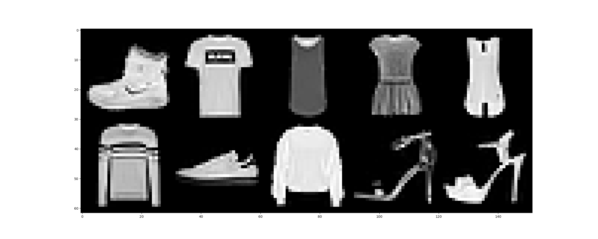

两段代码写的形式几乎一样，只有细微的差别。大家可以在Pycharm或者VSCode中分栏看一看这两段代码的区别。

(3) How to Plot Images Using PyTorch DataLoader

这一部分其实就是更复杂一点的应用，没啥特别需要注意的，直接贴代码放结果：

python 复制代码

import torch
import torchvision
import torchvision.transforms as transforms
import matplotlib.pyplot as plt

train_set = torchvision.datasets.FashionMNIST(
    root='./data'
    , train=True
    , download=True
    , transform=transforms.Compose([
        transforms.ToTensor()
    ])
)

how_many_to_plot = 20

train_loader = torch.utils.data.DataLoader(
    train_set, batch_size=1, shuffle=True
)

plt.figure(figsize=(40,25))
for i, batch in enumerate(train_loader, start=1):
    image, label = batch
    plt.subplot(5,5,i)
    plt.imshow(image.reshape(28,28), cmap='gray')
    plt.axis('off')
    plt.title(train_set.classes[label.item()], fontsize=28)
    if i >= how_many_to_plot: break
plt.show()

2.Section 2: Neural Networks and PyTorch Design

Bird's eye view of the process

From a high-level perspective or bird's eye view of our deep learning project, we prepared our data, and now, we are ready to build our model.

Prepare the data
Build the model
Train the model
Analyze the model's results

When say model , we mean our network . The words model and network mean the same thing. What we want our network to ultimately do is model or approximate a function that maps image inputs to the correct output class.

原作提到建议看deep learning fundamentals series这个系列课程作为入门，如果不看这个系列的全部课程也至少要看这5节：

If you just want a crash course on CNNs, these are the specific posts to see:

访问了一下他这个系列课程的博客，他推荐学习的是这5节：

贴一下全系列课程视频的网址：Deep Learning playlist overview & Machine Learning intro (youtube.com)

其实现在可以先不看这几个视频，我的思路是先学着，遇到问题之后再有针对性地看。当然了，如果你想现在就看这些视频也无伤大雅。

2.1.Build PyTorch CNN - Object Oriented Neural Networks

(1) Quick object oriented programming review

I recommend watching the explanation in the video: 17-Build PyTorch CNN - Object Oriented Neural Networks_哔哩哔哩_bilibili(from 01:44 to 09:30)

And the note: 囫囵吞枣学Python(1)------类-CSDN博客

(2) Building a neural network in PyTorch

Today we need to understand two words: layer and forward method.

So, first: What is layer?

layer:
- a transformation(using code)
- a collection of weights(using data)

Layers in PyTorch are defined by classes, so in code, our layers will be objects.(In the note: 囫囵吞枣学Python(1)------类-CSDN博客, the Students is defined by class, so the student1 is an object. If you don't understand, I suggest you review the first part: Quick object oriented programming review)

Second: What is forward method?

When we pass a tensor to our network as input, the tensor flows forward though each layer transformation until the tensor reaches the output layer. This process of a tensor flowing forward though the network is known as a forward pass.

The package torch.nn includes large number of classes and methods that we can use them directly.

First, Let's create a simple class to represent a neural network:

python 复制代码

class Network:
    def __init__(self):
        self.layer = None

    def forward(self, t):
        t = self.layer(t)
        return t

Second, Make our Network class extend nn.Module:

python 复制代码

import torch.nn as nn

class Network(nn.Module): # line 1
    def __init__(self):
        super().__init__() # line 3
        self.layer = None

    def forward(self, t):
        t = self.layer(t)
        return t

Both of these two parts of code have a characteristic commonly: the layer is empty. Now let's replace the None with some real layers which we will often use:

python 复制代码

import torch.nn as nn

class Network(nn.Module):
    def __init__(self):
        super().__init__()
        self.conv1 = nn.Conv2d(in_channels=1, out_channels=6, kernel_size=5)
        self.conv2 = nn.Conv2d(in_channels=6, out_channels=12, kernel_size=5)

        self.fc1 = nn.Linear(in_features=12 * 4 * 4, out_features=120)
        self.fc2 = nn.Linear(in_features=120, out_features=60)
        self.out = nn.Linear(in_features=60, out_features=10)

    def forward(self, t):
        # implement the forward pass
        return t

Conv2d: convolutional layers;
Linear: linear layers; linear layers are also called fully connected layers , and they also have a third name that we may hear sometimes called dense; so linear, dense, and fully connected are all ways to refer to the same type of layer;
We used the name out for the last linear layer because the last layer in the network is the output layer;

That is the end of this post, it's perfectly normal if you don't understand this part of code thoroughly. Don't worry about that. Just continue to learn with this doubt in mind, and you will gradually understand it.

2.2.CNN Layers - Deep Neural Network Architecture

Our goal in this post is to better understand the layers we have defined. To do this, we're going to learn about the parameters and the values that we passed for these parameters in the layer constructors.

(1) Parameter vs Argument

Parameters are used in function definitions. For this reason, we can think of parameters as place-holders.

Arguments are the actual values that are passed to the function when the function is called.

In our Network's case, the names like in_channels and out_channels are the parameters, and the values that we have specified like 1 and 6 are the arguments.

python 复制代码

import torch.nn as nn

class Network(nn.Module):
    def __init__(self):
        super().__init__()
        self.conv1 = nn.Conv2d(in_channels=1, out_channels=6, kernel_size=5)
        self.conv2 = nn.Conv2d(in_channels=6, out_channels=12, kernel_size=5)

        self.fc1 = nn.Linear(in_features=12 * 4 * 4, out_features=120)
        self.fc2 = nn.Linear(in_features=120, out_features=60)
        self.out = nn.Linear(in_features=60, out_features=10)

    def forward(self, t):
        # implement the forward pass
        return t

(2) Two types of parameters

Hyperparameters
Data dependent hyperparameters

In fact, a lot of terms in deep learning are used loosely(宽松地), and the word parameter is one of them. Try not to let it throw you off(使你困惑或分心，使你偏离正确的方向或计划).

In other words, these terms are not as important as you imagine.

Hyperparameters

Hyperparameters are parameters whose values are chosen manually(手动地) and arbitrarily(随意地). As neural network programmers, we choose hyperparameter values mainly based on trial(试验) and error and increasingly by utilizing(利用) values that have proven to work well in the past.

Talk like a human being, we usually test and tune(调整) these parameters to find values that work best.

In our Network's case, the parameters kernel_size, out_channels and out_features are hyperparameters(with a exception, the last out_features isn't a hyperparameter).

Parameter	Description
`kernel_size`	Sets the height and width of the filter.
`out_channels`	Sets depth of the filter. This is the number of kernels inside the filter. One kernel produces one output channel.
`out_features`	Sets the size of the output tensor.

One pattern that shows up quite often is that we increase our out_channels as we add additional convolutional layers, and after we switch to linear layers we shrink our out_features as we filter down to our number of output classes. We'll dive deeper into this in the next post.

Data dependent hyperparameters

Data dependent hyperparameters are parameters whose values are dependent on data.

Two typical parameters are the in_channels of the first convolutional layer, and the out_features of the output layer. The in_channels of the first convolutional layer depend on the number of color channels present inside the images that make up the training set. Since we are dealing with grayscale images, we know that this value should be a 1. The out_features for the output layer depend on the number of classes that are present inside our training set. Since we have 10 classes of clothing inside the Fashion-MNIST dataset, we know that we need 10 output features.

In general, the input to one layer is the output from the previous layer, and so all of the in_channels in the convolutional layers and in_features in the linear layers depend on the data coming from the previous layer.

Why we have 12*4*4? The 12 comes from the number of output channels in the previous layer, but why do we have the two 4s? We cover how we get these values in a future post.

(3) Descriptions of parameters

Layer	Param name	Param value	The param value is
conv1	in_channels	1	the number of color channels in the input image.
conv1	kernel_size	5	a hyperparameter.
conv1	out_channels	6	a hyperparameter.
conv2	in_channels	6	the number of out_channels in previous layer.
conv2	kernel_size	5	a hyperparameter.
conv2	out_channels	12	a hyperparameter (higher than previous conv layer).
fc1	in_features	1244	the length of the flattened output from previous layer.
fc1	out_features	120	a hyperparameter.
fc2	in_features	120	the number of out_features of previous layer.
fc2	out_features	60	a hyperparameter (lower than previous linear layer).
out	in_features	60	the number of out_channels in previous layer.
out	out_features	10	the number of prediction classes.

(4) Kernel vs Filter

We often use the words filter and kernel interchangeably(交替地) in deep learning. However, there is a technical distinction between these two concepts.

A kernel is a 2D tensor, and a filter is a 3D tensor that contains a collection of kernels. We apply a kernel to a single channel, and we apply a filter to multiple channels.

Reference: neural networks - Difference between "kernel" and "filter" in CNN - Cross Validated (stackexchange.com)

2.3.CNN Weights - Learnable Parameters in Neural Networks

(1) Another type of parameters

Learnable parameters

Learnable parameters are parameters whose values are learned during the training process. With learnable parameters, we typically start out with a set of arbitrary(任意的) values, and these values then get updated in an iterative(迭代的) fashion(方式) as the network learns.

In fact, when we say that a network is learning, we specifically mean that the network is learning the appropriate values for the learnable parameters.

(2) Getting an Instance the Network

python 复制代码

import torch.nn as nn

class Network(nn.Module):
    def __init__(self):
        super().__init__()
        self.conv1 = nn.Conv2d(in_channels=1, out_channels=6, kernel_size=5)
        self.conv2 = nn.Conv2d(in_channels=6, out_channels=12, kernel_size=5)

        self.fc1 = nn.Linear(in_features=12 * 4 * 4, out_features=120)
        self.fc2 = nn.Linear(in_features=120, out_features=60)
        self.out = nn.Linear(in_features=60, out_features=10)

    def forward(self, t):
        # implement the forward pass
        return t

network=Network()

print(network)

Result:

Network(
  (conv1): Conv2d(1, 6, kernel_size=(5, 5), stride=(1, 1))
  (conv2): Conv2d(6, 12, kernel_size=(5, 5), stride=(1, 1))
  (fc1): Linear(in_features=192, out_features=120, bias=True)
  (fc2): Linear(in_features=120, out_features=60, bias=True)
  (out): Linear(in_features=60, out_features=10, bias=True)
)

For the convolutional layers, the kernel_size argument is a Python tuple (5,5) even though we only passed the number 5 in the constructor. This is because our filters actually have a height and width, and when we pass a single number, the code inside the layer's constructor assumes that we want a square filter.

The stride is an additional parameter that we could have set, but we left it out. When the stride is not specified in the layer constructor the layer automatically sets it. The stride tells the conv layer how far the filter should slide after each operation in the overall convolution. This tuple says to slide by one unit when moving to the right and also by one unit when moving down.

For the linear layers, we have an additional parameter called bias which has a default parameter value of true. It is possible to turn this off by setting it to false.

In the video, the author also mentioned the word 'override'. We call it '重写' in Chinese. It's not important to focus on it here, so we don't have to worry about it.

(3) Accessing the Network's Layers

python 复制代码

print(network.conv1)
print(network.conv2)
print(network.fc1)
print(network.fc2)
print(network.out)

Result:

Conv2d(1, 6, kernel_size=(5, 5), stride=(1, 1))
Conv2d(6, 12, kernel_size=(5, 5), stride=(1, 1))
Linear(in_features=192, out_features=120, bias=True)
Linear(in_features=120, out_features=60, bias=True)
Linear(in_features=60, out_features=10, bias=True)

(4) Accessing the Layer Weights

Let's first look at some examples.

First, convolutional layers:

python 复制代码

import torch.nn as nn

class Network(nn.Module):
    def __init__(self):
        super().__init__()
        self.conv1 = nn.Conv2d(in_channels=1, out_channels=6, kernel_size=5)
        self.conv2 = nn.Conv2d(in_channels=6, out_channels=12, kernel_size=5)

        self.fc1 = nn.Linear(in_features=12 * 4 * 4, out_features=120)
        self.fc2 = nn.Linear(in_features=120, out_features=60)
        self.out = nn.Linear(in_features=60, out_features=10)

    def forward(self, t):
        # implement the forward pass
        return t

network=Network()

print(network.conv1)
print(network.conv1.weight)
print(network.conv1.weight.shape)

Result:

Conv2d(1, 6, kernel_size=(5, 5), stride=(1, 1))


Parameter containing:
tensor([[[[ 0.1232,  0.1745, -0.0915,  0.0615,  0.1538],
          [-0.0747, -0.0346,  0.0290, -0.0959,  0.0164],
          [ 0.0145, -0.0813, -0.1848, -0.1106, -0.1396],
          [-0.1269, -0.0738, -0.0959, -0.1527,  0.0644],
          [ 0.1800, -0.0883, -0.0080,  0.1344,  0.0920]]],

        [[[-0.0629,  0.1750, -0.1389,  0.1275, -0.1797],
          [-0.1755,  0.1946, -0.1925,  0.0654, -0.1339],
          [-0.1237, -0.1942, -0.1812, -0.1883,  0.1600],
          [ 0.1417,  0.1051,  0.1502, -0.1608, -0.1157],
          [ 0.0644,  0.1915, -0.1855,  0.1809, -0.0025]]],

        [[[ 0.1701, -0.0435, -0.1149, -0.0337,  0.0830],
          [ 0.0006,  0.0686,  0.1429, -0.1244, -0.0048],
          [ 0.0632, -0.1001,  0.1045, -0.1651,  0.1013],
          [ 0.1934,  0.1950, -0.0350,  0.0422, -0.0931],
          [-0.1226, -0.1583,  0.1330,  0.1100, -0.1544]]],

        [[[-0.0572, -0.0689,  0.1695,  0.0712,  0.0893],
          [ 0.1183, -0.0032, -0.0855,  0.0300,  0.0392],
          [-0.1271, -0.0850, -0.1440, -0.0717,  0.1915],
          [-0.0673, -0.1499,  0.0396,  0.1853, -0.1650],
          [ 0.1341, -0.1745, -0.1512,  0.1500, -0.1642]]],

        [[[-0.0190,  0.0146, -0.1059, -0.0617, -0.0630],
          [ 0.0148, -0.1553,  0.0026,  0.1763,  0.0672],
          [-0.1689,  0.1345,  0.1268,  0.1737,  0.1519],
          [ 0.1675, -0.0937, -0.0181,  0.0267, -0.0231],
          [-0.1085,  0.0345, -0.0552,  0.0690, -0.0950]]],

        [[[ 0.0343, -0.1318,  0.0569,  0.1160, -0.1973],
          [-0.0326,  0.1682,  0.1729, -0.0455, -0.0761],
          [-0.0124,  0.1356,  0.1893, -0.0778,  0.0509],
          [-0.1544, -0.0527,  0.1602,  0.1525,  0.0864],
          [ 0.0832,  0.1645,  0.1838,  0.1726, -0.1858]]]], requires_grad=True)


torch.Size([6, 1, 5, 5])

If we make some changes to the code:

python 复制代码

import torch.nn as nn

class Network(nn.Module):
    def __init__(self):
        super().__init__()
        self.conv1 = nn.Conv2d(in_channels=1, out_channels=6, kernel_size=5)
        self.conv2 = nn.Conv2d(in_channels=6, out_channels=12, kernel_size=5)

        self.fc1 = nn.Linear(in_features=12 * 4 * 4, out_features=120)
        self.fc2 = nn.Linear(in_features=120, out_features=60)
        self.out = nn.Linear(in_features=60, out_features=10)

    def forward(self, t):
        # implement the forward pass
        return t

network=Network()

print(network.conv2)
print(network.conv2.weight)
print(network.conv2.weight.shape)

Result:

Conv2d(6, 12, kernel_size=(5, 5), stride=(1, 1))


Parameter containing:
tensor([[[[-4.2884e-02, -1.8646e-02, -3.6468e-02, -2.1878e-02, -6.1812e-02],
          [ 2.9104e-02,  4.3656e-02,  2.1134e-02,  6.8243e-02,  3.9659e-02],
          [-4.8924e-02,  5.9818e-02, -3.0731e-02,  3.9902e-02, -9.6543e-03],
          [ 4.2226e-03,  7.7117e-02, -5.0710e-02,  7.5835e-02, -7.0011e-02],
          [ 2.4738e-02, -7.1612e-03, -6.5956e-02, -7.1910e-02, -4.0692e-03]],

         [[ 5.9244e-02, -5.4084e-02, -4.1429e-02, -5.3655e-02, -2.9016e-02],
          [ 5.7895e-02,  1.6712e-02, -5.7220e-02,  2.0745e-02,  7.3740e-02],
          [ 6.4129e-02,  4.3146e-02,  2.0793e-02,  4.8607e-02, -1.8870e-02],
          [-1.8324e-02, -6.2051e-02, -4.5263e-02,  3.0059e-02,  2.4538e-02],
          [ 2.5017e-02, -6.1615e-02, -1.4608e-02, -2.3294e-02, -1.0028e-02]],

         [[ 3.9857e-02, -6.9648e-02, -4.9927e-02,  7.9932e-03, -6.4465e-02],
          [-3.1335e-02,  4.7432e-02,  1.8392e-02, -9.7926e-03,  7.6205e-02],
          [ 5.1769e-02, -3.8508e-02,  2.1279e-02,  5.8801e-02, -7.6870e-02],
          [ 6.5906e-02, -6.5944e-02,  6.4801e-02, -5.0759e-02, -2.9017e-02],
          [ 5.1388e-02,  3.3068e-02,  5.1049e-02,  8.1391e-02,  5.6871e-02]],

         [[ 7.6068e-03,  5.7764e-02,  1.3304e-02,  2.3320e-02,  7.1435e-02],
          [ 6.1237e-02,  2.0400e-02,  2.8379e-05,  7.6489e-02,  7.2457e-02],
          [ 9.6467e-03, -1.4250e-02, -7.3180e-02, -2.4022e-02, -2.0675e-02],
          [-5.6530e-02, -4.8809e-03,  2.8938e-02,  7.1006e-02, -4.4209e-02],
          [-2.6500e-02, -3.5677e-03,  6.7954e-02, -3.1715e-02,  5.1770e-02]],

         [[ 1.3207e-02,  3.0945e-02, -7.3218e-02,  5.3696e-02, -5.5415e-02],
          [ 6.4929e-02, -3.0792e-02, -2.1799e-02,  4.3814e-02,  6.4807e-02],
          [-1.4082e-02, -1.2352e-02, -4.1357e-02, -5.0738e-02, -1.2696e-02],
          [ 2.3784e-02,  4.4909e-02, -5.8380e-02,  6.7909e-02, -8.2366e-03],
          [-7.9928e-02,  3.4381e-02, -5.9752e-02, -7.8087e-02,  2.9481e-02]],

         [[ 2.8638e-02, -6.7411e-02,  4.7579e-02,  1.0333e-02,  6.7232e-02],
          [ 4.3504e-02,  5.4487e-02,  5.1175e-02, -6.6485e-03,  6.6359e-02],
          [ 3.0006e-02,  6.1103e-02, -2.9882e-02, -6.9170e-02, -3.3795e-02],
          [ 5.4645e-02,  5.9930e-02,  7.2578e-02, -3.9443e-02,  5.6268e-02],
          [-6.5664e-04, -3.5357e-02,  6.3044e-02,  2.8497e-02, -4.8495e-02]]],


        [[[-1.5204e-02, -2.0982e-04,  5.2414e-02,  6.6475e-02, -3.9259e-02],
          [ 1.8214e-02,  4.8985e-02, -1.5981e-02, -3.1356e-02, -7.6915e-03],
          [-1.8750e-02, -2.3607e-02, -2.1833e-02,  7.7038e-02, -4.7328e-02],
          [-4.3814e-02, -4.0106e-02,  3.3002e-02,  7.4004e-02,  7.5722e-02],
          [ 3.9917e-02, -3.7348e-02, -6.0048e-02,  2.1473e-02, -5.3794e-02]],

         [[-6.9337e-02, -6.3384e-02, -7.8037e-02,  2.7754e-02,  4.9844e-02],
          [-1.8384e-02,  8.1333e-02,  8.1422e-02, -2.4105e-03, -6.8615e-02],
          [-4.6947e-02, -5.5351e-02,  4.5957e-02,  2.9277e-02, -1.3860e-02],
          [-4.6693e-02,  2.8683e-02,  6.1394e-02,  8.0850e-02, -5.0913e-02],
          [ 5.7079e-02,  6.9726e-02, -7.1289e-03,  6.4266e-04,  5.3523e-02]],

         [[-2.6457e-03, -2.0547e-02, -7.2038e-02, -2.7709e-02, -6.1851e-02],
          [-4.1947e-02,  3.4758e-02,  2.2606e-02, -5.2566e-02,  8.0384e-02],
          [-3.1233e-02, -4.4558e-02,  8.4542e-03,  3.6306e-02, -8.1493e-02],
          [ 1.7083e-02,  8.3195e-04, -7.9616e-02,  2.9549e-03, -5.3943e-02],
          [ 3.2066e-02,  7.3952e-03,  1.1623e-02, -5.5744e-02,  1.7965e-02]],

         [[ 5.3836e-02, -6.7208e-02, -6.1651e-02, -1.8709e-02,  5.6753e-02],
          [ 8.2612e-03, -3.2186e-02, -2.6628e-02, -4.6597e-02, -7.2020e-02],
          [-4.3285e-03,  1.1460e-02, -3.0413e-02,  5.2102e-02, -7.5177e-02],
          [-7.1347e-02,  5.5588e-02,  6.9111e-02,  1.4323e-02, -5.7546e-02],
          [-1.8687e-02, -7.7605e-02, -8.0353e-02, -3.2596e-02, -3.1418e-02]],

         [[-6.9735e-02,  5.3523e-02, -5.3416e-02,  4.5771e-02,  5.6954e-02],
          [ 6.3120e-02,  5.5763e-02,  1.6067e-02,  8.6567e-03, -4.2644e-02],
          [-5.9344e-02, -4.6653e-03,  7.6593e-02, -7.3292e-02, -5.3917e-02],
          [ 6.6566e-02,  3.1131e-02,  7.7349e-02, -2.7129e-02,  8.4518e-03],
          [ 1.6985e-02, -7.0555e-02,  3.8170e-02, -1.1612e-02, -7.6542e-02]],

         [[-6.0196e-02, -6.4580e-02, -3.1164e-03, -4.1933e-02,  7.1420e-03],
          [ 7.9487e-02, -1.4821e-02,  2.2844e-03, -1.5251e-03,  3.7557e-02],
          [-6.8896e-02, -6.6881e-03,  5.7520e-02,  1.8301e-02, -3.7004e-02],
          [-2.5592e-02,  3.0609e-02,  6.9578e-02,  5.5549e-02, -5.3245e-02],
          [ 4.6727e-02,  8.0116e-02, -7.5505e-02, -2.8765e-02, -3.5874e-02]]],


        [[[ 5.3670e-02,  7.4484e-02, -6.3226e-02, -2.9761e-02,  6.0873e-02],
          [-6.1811e-02,  1.6729e-02,  4.5729e-02,  2.8226e-04, -1.3171e-02],
          [-1.2364e-02,  7.2936e-02,  1.0765e-02,  3.1374e-02,  1.7582e-02],
          [ 1.3305e-02, -6.6938e-02, -6.6351e-02,  4.8234e-02,  2.5997e-02],
          [-4.1954e-03, -6.4869e-02,  1.7950e-02,  3.3482e-02, -1.2225e-02]],

         [[-1.3839e-02,  3.9010e-02, -6.4779e-02, -7.0044e-02, -2.7837e-02],
          [ 5.8636e-02,  7.5278e-02,  7.1607e-02,  5.5469e-02,  5.4468e-02],
          [-7.4318e-02,  7.4283e-03, -2.3738e-02,  6.4434e-02,  1.9524e-02],
          [ 7.8238e-02,  5.3939e-02, -4.3555e-02,  6.3559e-02,  8.1849e-04],
          [-5.5254e-02, -6.8373e-02,  5.0078e-02,  2.6748e-02,  4.5676e-02]],

         [[ 7.1268e-02,  3.6513e-03,  2.4753e-02,  3.5536e-02,  2.0245e-02],
          [ 5.9411e-02,  6.5015e-02,  6.7302e-02,  5.5706e-02, -7.3357e-02],
          [ 6.7356e-02,  2.8092e-02,  8.0472e-02,  6.9567e-02, -3.6824e-02],
          [-4.3014e-02, -7.9176e-02,  5.1021e-02, -3.2842e-02,  4.3498e-02],
          [-3.7790e-03,  3.6721e-03,  3.3520e-02,  3.8218e-02, -6.1545e-02]],

         [[-4.7160e-02, -2.7351e-02, -6.6609e-02, -6.4513e-03,  3.4438e-02],
          [-4.4675e-03, -6.5095e-02,  6.1610e-02,  8.0325e-02,  5.7229e-02],
          [-1.3750e-02, -1.0938e-02, -4.5011e-02,  6.9686e-02,  5.1559e-02],
          [ 5.8902e-02, -1.1045e-02, -4.3365e-02, -2.8516e-04,  7.0693e-02],
          [ 5.4149e-02, -3.4944e-02, -4.5348e-02, -4.7880e-02, -6.0826e-02]],

         [[ 8.4448e-03,  9.3816e-03,  3.4866e-02,  3.8719e-04, -4.4713e-02],
          [-3.7519e-02,  1.4705e-02,  3.1401e-02,  6.1778e-02, -2.9698e-02],
          [ 2.0491e-02, -1.3609e-02,  6.7055e-02,  4.1654e-02, -3.3637e-02],
          [-6.8364e-02, -5.5866e-02, -7.7622e-02,  1.5276e-02, -3.5520e-02],
          [ 3.1254e-02, -7.0029e-02,  4.4888e-02,  5.9723e-02,  3.6382e-02]],

         [[-2.3066e-02,  6.7966e-02,  5.1811e-02, -5.9159e-02,  3.1069e-02],
          [ 5.1321e-02,  6.7464e-02,  7.5866e-02, -5.5414e-02,  4.0420e-02],
          [-4.4354e-02,  7.9306e-02, -1.4644e-02, -9.3875e-03,  2.6070e-02],
          [ 7.4850e-02,  6.0425e-02, -2.0909e-02,  5.9285e-02,  4.6566e-02],
          [ 1.3756e-02,  1.1649e-02,  2.8588e-02, -1.3022e-03,  2.3256e-02]]],


        ...,


        [[[ 7.6311e-02,  7.5261e-02,  5.7561e-02, -4.3356e-02, -7.2909e-02],
          [-4.6708e-02,  5.1551e-02, -4.8101e-02, -5.1413e-02, -3.6152e-02],
          [ 6.0626e-02,  5.6325e-04, -2.1743e-02,  3.3400e-02,  7.9141e-02],
          [ 3.5604e-02,  6.9508e-02, -2.1984e-02,  5.9585e-02, -9.4945e-03],
          [-4.0188e-02, -5.4732e-03,  6.8583e-02,  3.0551e-02, -1.1802e-02]],

         [[ 5.2653e-02,  6.1670e-02,  2.6309e-03,  5.3165e-02, -3.8166e-02],
          [ 8.1076e-02,  5.7386e-02, -6.1753e-02,  4.9131e-02,  3.6430e-02],
          [-4.7202e-02, -4.2705e-02, -4.6333e-02,  6.7525e-02,  4.8547e-02],
          [ 7.9853e-02, -8.0172e-02,  4.9944e-03, -5.7631e-02, -6.1132e-03],
          [-5.5667e-03, -2.1569e-02, -2.8139e-02, -8.9662e-03,  3.5014e-02]],

         [[-3.0472e-02,  3.0703e-02,  5.1314e-02, -6.2341e-02, -6.3894e-02],
          [-7.6258e-02,  1.6020e-02,  3.3108e-02, -6.8395e-02, -5.7936e-02],
          [ 6.3067e-02,  6.1881e-04, -8.0695e-02, -1.7197e-02,  2.2778e-02],
          [ 4.4634e-02, -7.0455e-02, -2.1533e-02,  3.6857e-02,  5.7196e-02],
          [ 3.5345e-02,  6.9631e-02,  5.5229e-02,  4.2128e-02, -3.4088e-02]],

         [[-7.2163e-03,  3.5563e-02, -3.1936e-02,  1.2877e-02, -2.3022e-02],
          [-5.9097e-02,  1.5192e-02,  6.8320e-02, -4.6643e-02, -1.9811e-03],
          [-5.9560e-03,  7.7662e-02,  7.9657e-02, -4.4968e-02, -7.6457e-02],
          [-1.1028e-02, -3.5175e-02, -1.3390e-02,  5.1161e-02, -5.4926e-02],
          [-4.1221e-02,  6.2617e-02, -5.9798e-02, -8.9769e-04,  6.3048e-02]],

         [[ 4.4751e-02, -5.1591e-02, -3.6866e-02, -7.4997e-02,  4.9472e-02],
          [-6.2221e-02,  6.6295e-02, -5.0621e-02,  3.4758e-02, -2.1337e-02],
          [ 5.0706e-02, -5.2147e-02,  6.8346e-02,  3.2746e-02,  7.1333e-02],
          [-1.4602e-02, -6.2453e-02, -1.9406e-02,  6.9041e-02, -2.8379e-02],
          [ 3.4721e-03,  7.7462e-02,  5.1289e-02,  3.3926e-02, -2.8289e-02]],

         [[-5.0928e-02, -2.8340e-02,  2.2817e-02,  7.0458e-02,  4.2438e-02],
          [-3.3680e-02,  4.5647e-02, -4.9270e-02, -2.8433e-02,  2.9541e-02],
          [ 2.3391e-02, -7.4426e-02,  6.4900e-02, -7.1001e-02,  4.5884e-02],
          [-5.7277e-02, -4.6285e-03,  5.3839e-02, -5.6219e-02,  7.9665e-02],
          [-8.1319e-02, -8.1240e-02,  1.2502e-02,  5.5328e-02,  2.0030e-02]]],


        [[[ 4.8441e-02,  4.8989e-02, -2.4322e-02, -5.9358e-02, -6.8357e-02],
          [-2.1089e-02,  4.5388e-02, -5.1134e-03,  4.3126e-02, -1.6892e-03],
          [-8.1167e-02, -5.7231e-02,  3.9827e-02, -6.3646e-03, -3.9094e-02],
          [-4.2316e-02,  5.3464e-02, -8.8957e-03, -4.7075e-02, -1.7774e-02],
          [-6.5931e-02,  1.1694e-02, -3.9309e-02,  4.1809e-02,  1.2976e-03]],

         [[-6.8713e-02, -1.7812e-02, -1.4486e-02,  8.3056e-03, -6.8082e-02],
          [-1.8569e-02,  2.6123e-02,  2.4870e-05,  5.6066e-02,  4.5435e-02],
          [ 5.3947e-02,  1.4763e-02,  1.4906e-02, -5.5155e-02,  4.7769e-02],
          [ 5.3297e-02, -3.9101e-02,  4.6465e-02,  1.1151e-02,  5.5033e-02],
          [ 3.6748e-03,  3.9723e-02, -4.1154e-02,  4.6245e-02, -3.3245e-02]],

         [[-1.8014e-02, -8.0139e-02, -6.3273e-03, -3.8566e-02,  4.0923e-03],
          [ 5.8483e-02, -6.5439e-02,  2.0173e-02,  7.2705e-02, -3.5129e-02],
          [-4.8423e-02, -5.2663e-02, -1.3957e-02,  2.9158e-02,  7.8463e-02],
          [ 7.1398e-04,  6.5734e-02,  3.6854e-02, -2.1278e-02,  3.3324e-02],
          [ 3.6285e-02,  4.2179e-02, -2.9803e-02, -4.1720e-03, -2.0233e-02]],

         [[-2.7885e-02,  5.2520e-02,  5.1337e-02, -2.6349e-02,  1.5047e-02],
          [ 8.1576e-02, -3.3374e-02,  2.2938e-02, -4.8218e-02,  3.5318e-02],
          [-6.8747e-02, -4.1312e-02,  7.9037e-03,  6.8197e-02, -5.2138e-02],
          [ 2.2267e-03,  2.0724e-02, -5.1848e-02,  4.9394e-02,  7.5763e-02],
          [ 3.7441e-02,  2.7114e-02,  2.8150e-02, -5.4438e-02, -5.9701e-02]],

         [[ 7.5385e-02,  2.2393e-02, -6.8777e-02, -2.0514e-02,  6.8338e-02],
          [-6.6630e-02,  7.4462e-02,  4.0799e-02, -1.2080e-02,  7.0668e-02],
          [-7.2318e-03, -4.5113e-02, -8.0733e-03,  6.0332e-02,  7.7593e-02],
          [ 1.5821e-02, -2.2018e-02,  7.7987e-02,  4.0169e-02, -6.3680e-02],
          [-8.1590e-02,  6.3925e-02,  6.4027e-02,  3.3750e-02, -6.6571e-02]],

         [[-4.0221e-02,  2.1132e-02, -7.6372e-02,  3.1901e-02, -2.6639e-03],
          [ 6.2732e-02,  2.5971e-02, -3.8870e-02, -5.9896e-02,  3.6378e-02],
          [ 1.7306e-02,  4.8518e-02, -3.4341e-02, -5.0257e-03, -7.7493e-02],
          [-5.3312e-02,  4.5801e-02,  6.3797e-02, -7.6749e-02, -1.9681e-02],
          [ 4.9668e-02,  2.5340e-02, -4.5465e-02,  5.5866e-02, -1.7633e-03]]],


        [[[ 3.3887e-02,  4.1100e-02, -6.0800e-02,  3.0658e-02, -2.4294e-02],
          [ 2.2048e-02,  3.4223e-02, -2.1182e-02, -1.4165e-02,  2.0991e-02],
          [-3.8944e-03,  2.8239e-02, -3.5322e-02, -2.2963e-02,  2.2183e-02],
          [-4.6182e-02,  7.5100e-02, -5.7425e-02, -7.0277e-02,  7.4489e-02],
          [-6.5370e-02,  6.8510e-02,  2.4596e-02,  7.9349e-03,  4.1632e-02]],

         [[-8.0785e-02, -5.5982e-02, -5.2925e-02,  4.4351e-02, -5.4612e-02],
          [-2.7587e-02, -4.9968e-02,  4.6770e-02, -4.7240e-02,  5.7632e-02],
          [ 2.1552e-02,  1.9329e-03, -3.6635e-02, -4.1714e-04,  7.6460e-02],
          [ 8.0785e-02,  5.0883e-02,  7.0737e-02,  4.5160e-02,  1.2882e-03],
          [ 7.1417e-02, -2.8139e-02,  6.3305e-02, -2.5239e-02,  7.1895e-02]],

         [[-7.3631e-02, -3.3411e-02,  3.2707e-02, -6.8281e-02,  2.5994e-02],
          [ 5.2490e-02, -5.4156e-02, -8.1550e-02, -2.4794e-02, -6.3099e-02],
          [ 4.9664e-02,  1.6858e-02, -4.8651e-02,  1.4407e-02, -7.8078e-02],
          [ 8.1470e-03,  2.8146e-03,  5.2201e-02, -2.3638e-02, -3.0703e-02],
          [ 7.4847e-02, -2.3422e-02,  2.0211e-02, -3.9981e-02,  4.2893e-02]],

         [[-3.6386e-02,  6.5790e-02,  4.4377e-02, -3.0673e-02,  6.3339e-02],
          [-3.0514e-03,  6.0295e-02,  2.9729e-02, -4.2983e-02,  3.9292e-02],
          [ 3.1405e-02, -7.3552e-02,  3.4892e-03, -2.5254e-02,  8.5877e-03],
          [ 7.1609e-02, -5.1557e-02, -4.3620e-03, -1.5285e-02,  1.2429e-03],
          [ 6.9231e-02,  3.3598e-02,  2.8721e-02, -2.2294e-02, -7.9912e-02]],

         [[-7.5321e-03,  4.9022e-02, -8.0334e-02,  6.9277e-03, -7.5131e-02],
          [ 3.3288e-02,  7.3412e-03, -4.8152e-02, -7.9854e-02,  7.6142e-02],
          [-1.4706e-02,  5.5508e-02,  3.6131e-02,  7.8418e-02,  7.6000e-02],
          [ 2.8675e-02,  4.3452e-02, -5.0536e-02, -8.1299e-02, -4.2749e-02],
          [ 1.1211e-02, -5.1659e-02,  3.7996e-02, -1.3355e-02,  8.0545e-02]],

         [[-5.1144e-02, -2.0223e-02,  6.8809e-02, -5.1931e-02, -4.6908e-02],
          [ 7.0982e-02, -7.3319e-02, -7.8952e-02, -8.1581e-02, -5.7866e-02],
          [ 1.6373e-03, -6.2698e-02,  1.2726e-02,  5.8875e-02,  5.3699e-02],
          [-9.7808e-03, -2.1850e-02,  9.0736e-03, -5.3497e-02,  1.2925e-02],
          [ 2.4039e-02,  7.6288e-02, -2.5936e-03,  5.2908e-02, -6.6839e-02]]]],
       requires_grad=True)


torch.Size([12, 6, 5, 5])

It's obviously that the weight of a convolutional layer is a rank-4 tensor, and the shape of the tensor is [out_channels, in_channels, kernel_size, kernel_size].

其实weight tensor中，这些大小为5×5的weight就是这个kernel里面的内容，即filter。这是我们第一次如此直观地看这个5×5的玩意，所以为了更好地理解，需要好好学一学什么是卷积了。可以按顺序看一下这几个视频：

离散卷积：【官方双语】那么......什么是卷积？_哔哩哔哩_bilibili
连续卷积：【官方双语】卷积的两种可视化|概率论中的X+Y既美妙又复杂_哔哩哔哩_bilibili
图像处理中的卷积：Convolutional Neural Networks (CNNs) explained (youtube.com)

在conv1层中，由于我们随便将输出通道设置为6，所以如果我们想要得到6通道的输出，那么我们应该有6个不同的滤波器。及对应刚刚看到的network.conv1.weight.shape为[6,1,5,5]。先不管这里面这个1。

类比conv1层，是不是在conv2层中，由于我们又随便将输出通道设置为12，所以如果我们想要得到12通道的输出，应该有12个不同的滤波器呢？诶，但是这时候就发现了：如果是12个5×5的滤波器，那network.conv2.weight[0][0]、network.conv2.weight[1][0]、...、network.conv2.weight[11][0]的这12个5×5的张量不应该一样吗？岂不是应该叫有12×6个5×5的滤波器？

实际不然。在上述三个视频中，其动画演示均为二维图像、二维滤波器。然而实际上，这个滤波器可以是高维的。还是以刚刚的两层卷积为例：conv1时，一个5×5的滤波器滑过原始图形进行卷积，然后得到6张feature map；conv2时，这6张feature map像叠豆腐皮一样叠在一起，从俯视图来看，不论是滤波器还是feature map都还是二维的，然而要是从侧面看，那这6张feature map还有"高度"，这个滤波器也有"高度"，6张feature map的"高度"和这个俯视图大小为5×5的滤波器的"高度"一样，都是6。

理解了这个之后，我们再回看conv1，其实这个滤波器也不是严格意义上的二维，而是"高度"为1的三维。

当然了，这个"高度"也有更专业的叫法：depth。

As for linear layers:

python 复制代码

import torch.nn as nn

class Network(nn.Module):
    def __init__(self):
        super().__init__()
        self.conv1 = nn.Conv2d(in_channels=1, out_channels=6, kernel_size=5)
        self.conv2 = nn.Conv2d(in_channels=6, out_channels=12, kernel_size=5)

        self.fc1 = nn.Linear(in_features=12 * 4 * 4, out_features=120)
        self.fc2 = nn.Linear(in_features=120, out_features=60)
        self.out = nn.Linear(in_features=60, out_features=10)

    def forward(self, t):
        # implement the forward pass
        return t

network=Network()

print(network.fc1)
print(network.fc1.weight)
print(network.fc1.weight.shape)

Result:

Linear(in_features=192, out_features=120, bias=True)


Parameter containing:
tensor([[-0.0705,  0.0281, -0.0345,  ...,  0.0707,  0.0039,  0.0049],
        [ 0.0185, -0.0139, -0.0371,  ..., -0.0181,  0.0251, -0.0153],
        [-0.0564, -0.0413,  0.0650,  ..., -0.0377,  0.0203,  0.0308],
        ...,
        [-0.0158, -0.0176, -0.0564,  ...,  0.0637,  0.0659, -0.0601],
        [ 0.0695, -0.0088,  0.0561,  ..., -0.0145,  0.0285, -0.0415],
        [ 0.0472,  0.0183,  0.0253,  ...,  0.0290,  0.0631,  0.0598]],
       requires_grad=True)


torch.Size([120, 192])

If we make some changes to the code:

python 复制代码

import torch.nn as nn

class Network(nn.Module):
    def __init__(self):
        super().__init__()
        self.conv1 = nn.Conv2d(in_channels=1, out_channels=6, kernel_size=5)
        self.conv2 = nn.Conv2d(in_channels=6, out_channels=12, kernel_size=5)

        self.fc1 = nn.Linear(in_features=12 * 4 * 4, out_features=120)
        self.fc2 = nn.Linear(in_features=120, out_features=60)
        self.out = nn.Linear(in_features=60, out_features=10)

    def forward(self, t):
        # implement the forward pass
        return t

network=Network()

print(network.fc2)
print(network.fc2.weight)
print(network.fc2.weight.shape)

Result:

Linear(in_features=120, out_features=60, bias=True)


Parameter containing:
tensor([[-0.0125, -0.0863,  0.0814,  ...,  0.0540, -0.0659, -0.0135],
        [ 0.0179, -0.0563, -0.0102,  ..., -0.0826, -0.0142,  0.0196],
        [ 0.0842, -0.0230,  0.0686,  ..., -0.0196,  0.0216, -0.0474],
        ...,
        [-0.0725,  0.0761, -0.0251,  ..., -0.0715,  0.0418,  0.0547],
        [ 0.0271,  0.0791,  0.0274,  ..., -0.0206,  0.0681, -0.0490],
        [ 0.0534,  0.0316,  0.0514,  ..., -0.0452,  0.0563,  0.0776]],
       requires_grad=True)


torch.Size([60, 120])

If we make some changes to the code again:

python 复制代码

import torch.nn as nn

class Network(nn.Module):
    def __init__(self):
        super().__init__()
        self.conv1 = nn.Conv2d(in_channels=1, out_channels=6, kernel_size=5)
        self.conv2 = nn.Conv2d(in_channels=6, out_channels=12, kernel_size=5)

        self.fc1 = nn.Linear(in_features=12 * 4 * 4, out_features=120)
        self.fc2 = nn.Linear(in_features=120, out_features=60)
        self.out = nn.Linear(in_features=60, out_features=10)

    def forward(self, t):
        # implement the forward pass
        return t

network=Network()

print(network.out)
print(network.out.weight)
print(network.out.weight.shape)

Result:

Linear(in_features=60, out_features=10, bias=True)


Parameter containing:
tensor([[-9.5431e-02, -1.7005e-02,  7.1840e-02, -9.8549e-02, -7.6483e-02,
         -1.1399e-01, -7.4596e-02,  2.7645e-02,  4.7635e-02, -7.7890e-03,
         -1.2679e-01,  1.0586e-01, -3.0603e-02, -5.9335e-02,  2.3362e-02,
          1.2566e-01,  1.5932e-02,  6.4170e-02,  1.1894e-01,  1.1183e-02,
          5.5053e-02,  9.9240e-02,  9.1880e-02,  6.6743e-02, -1.9384e-02,
         -1.9155e-02,  4.9925e-02, -1.2826e-01,  4.2235e-02, -4.1539e-02,
          4.3719e-02,  1.1860e-02, -4.2918e-02,  6.8773e-02,  6.1953e-02,
          8.6118e-02,  7.6434e-02,  1.1209e-01, -2.3595e-02, -4.3001e-02,
          6.5224e-02,  1.2810e-01, -2.2255e-02, -1.4613e-02,  3.5808e-02,
          7.5827e-02,  9.4326e-02, -3.0887e-02, -4.9017e-02,  1.8240e-02,
          4.2232e-02, -1.0665e-01, -4.2260e-02,  4.7343e-02, -2.9680e-02,
          9.0191e-02,  2.2731e-02, -9.6192e-02, -6.2657e-02,  1.0931e-01],
        [ 1.0550e-01,  9.0423e-02, -9.3332e-02,  1.2436e-01,  3.2053e-02,
          8.7275e-02,  3.5335e-02,  9.3939e-02,  1.5199e-02,  5.1158e-02,
         -5.0064e-02,  9.0380e-02, -1.1103e-01,  2.5579e-02,  6.2949e-02,
          5.0965e-02,  1.8335e-02, -9.3640e-02,  4.6990e-02, -7.4176e-02,
         -1.0114e-01,  4.4343e-02, -1.1196e-01, -1.0231e-03, -9.9206e-03,
          6.2436e-02,  5.1555e-02,  1.0264e-01, -4.7560e-02,  1.1569e-01,
          5.7760e-02, -5.1481e-02,  3.1187e-02,  1.0843e-02,  1.6946e-03,
         -9.8104e-02,  1.2487e-01,  4.9549e-02, -6.4053e-02,  4.9612e-02,
          9.1507e-02,  9.7179e-02, -9.7871e-02,  6.7297e-02, -4.9381e-02,
         -3.8144e-02,  1.0243e-01,  3.2595e-02, -3.9338e-02,  1.1845e-01,
         -8.1794e-02,  9.7819e-02, -5.1667e-02, -1.1482e-01,  4.4470e-02,
         -2.8988e-03,  7.9396e-02, -7.8607e-02,  1.0526e-01, -4.2752e-02],
        [ 1.0955e-01,  4.8004e-02,  3.2397e-02,  3.4339e-02, -1.1132e-01,
          1.0589e-01,  8.7578e-02, -7.5346e-02, -2.3077e-02, -2.7315e-02,
          7.1867e-02, -8.9190e-02, -6.9571e-02, -2.3352e-04,  5.8229e-02,
         -2.1809e-03, -4.7928e-02,  9.5225e-02,  4.2706e-02,  1.0974e-01,
          1.1307e-01,  1.0599e-01, -2.3031e-02,  1.1409e-01, -4.7209e-02,
         -5.9337e-02, -9.2169e-02, -7.9493e-02, -6.5236e-02,  3.4885e-02,
          1.0364e-01,  1.1474e-01,  5.3987e-02, -9.2154e-02, -3.3679e-02,
          1.1838e-02,  1.4456e-02, -9.1507e-02, -1.0978e-02,  7.8048e-02,
         -1.7644e-02,  9.0853e-02,  5.6694e-02, -2.5896e-03, -6.1217e-02,
         -1.0350e-01,  4.4196e-02, -8.6999e-02,  9.8554e-02,  4.5385e-02,
         -1.2163e-01, -1.2214e-01,  1.1512e-01,  6.2625e-03,  1.2238e-02,
         -1.2423e-01,  1.1331e-01, -1.2531e-01,  8.2710e-02, -4.4940e-02],
        [-3.0085e-02,  3.8706e-02,  8.4378e-02, -5.4317e-02,  3.9812e-03,
         -1.0402e-01,  1.0845e-01, -8.3468e-02, -7.2716e-02, -6.2164e-02,
         -6.5018e-02,  1.0793e-01, -3.2918e-02,  5.4166e-05, -7.5525e-02,
          5.7055e-02, -7.7655e-02, -8.9118e-02,  9.4000e-02, -1.0995e-01,
         -1.2352e-01, -5.9220e-02, -8.2974e-02, -5.7302e-02,  1.5609e-02,
         -1.2284e-01,  6.3260e-03, -7.5324e-02,  8.5237e-02,  1.1582e-01,
          2.7184e-03,  9.7957e-02,  9.8548e-02, -3.8990e-02, -1.1632e-01,
         -4.2078e-02, -1.2860e-01,  3.8189e-02, -4.3375e-02,  8.3966e-03,
          7.8744e-02,  6.0847e-02,  3.0520e-02, -1.0597e-01, -4.5798e-03,
         -2.7219e-02,  9.6288e-02,  5.9863e-02,  4.3751e-02, -8.4328e-02,
         -6.4868e-02,  2.6567e-02, -1.5164e-02,  1.0628e-01,  2.0222e-02,
          7.9692e-02,  1.2675e-01, -6.1683e-02,  8.6366e-02, -9.7108e-02],
        [ 5.2049e-02,  5.8477e-02, -2.1854e-02,  1.1417e-01,  3.6167e-02,
          8.5150e-02,  7.1177e-02, -1.0457e-01, -4.9616e-02,  1.1462e-01,
          1.2540e-01, -1.1023e-01, -1.4444e-02,  8.2458e-02,  4.3347e-02,
          2.1713e-02,  4.5096e-02, -8.6695e-02, -1.1800e-01, -3.4499e-02,
         -3.3037e-02,  6.5183e-02, -5.5824e-02, -1.7711e-02, -3.2948e-02,
          3.7119e-02,  3.9931e-02,  8.4765e-02, -1.1503e-02, -1.0770e-01,
          9.0663e-02,  2.4122e-04,  3.0893e-02, -9.9923e-02,  7.0852e-02,
         -1.0870e-01,  1.9549e-02,  1.0645e-02,  4.2231e-02, -1.3988e-02,
          1.0743e-01, -4.0840e-02,  3.7030e-02, -1.9841e-02,  1.2380e-01,
          1.0932e-01,  9.7837e-02, -4.2590e-02,  3.5842e-02, -5.3193e-02,
         -1.1814e-01,  1.0496e-01,  9.8266e-02, -5.5253e-02, -7.5407e-02,
         -1.2650e-01, -1.0021e-01, -4.8345e-02, -7.2046e-02, -1.1478e-01],
        [ 1.0777e-01,  5.4178e-02,  3.9708e-02,  2.1861e-02,  1.5687e-02,
          5.2035e-02,  7.5276e-02, -1.0342e-01, -1.2357e-01,  9.8690e-03,
          6.1068e-02,  5.2973e-02, -4.8771e-02,  4.1235e-02,  1.0646e-01,
          5.7729e-02, -1.2204e-01, -5.1925e-02, -1.0611e-01,  5.0993e-02,
          1.2388e-01, -2.8327e-02,  1.1061e-01,  9.8941e-02, -8.1721e-02,
         -1.2586e-01, -6.6573e-02,  1.2495e-01, -9.1882e-02,  1.4345e-02,
         -3.7698e-02,  9.5678e-02, -8.9728e-02, -1.2532e-01, -6.8664e-02,
         -1.0077e-01, -1.2485e-01, -1.0039e-01,  1.7366e-02, -9.2025e-02,
         -1.2193e-01,  8.4152e-02,  1.1543e-01, -1.5280e-04, -5.1611e-03,
          9.3243e-02, -6.9181e-02,  1.1578e-01,  1.2789e-01,  8.4413e-02,
         -1.2359e-01,  1.2410e-01,  5.4242e-02, -4.2676e-02,  8.6314e-02,
         -1.2145e-01, -4.4658e-02,  1.0574e-01, -1.1472e-01,  6.9706e-02],
        [ 6.5161e-03,  5.0922e-02, -5.6269e-02, -3.0558e-02,  3.1047e-02,
          9.0965e-02, -1.1643e-01, -8.0907e-02, -1.1244e-02, -8.4535e-02,
          2.2675e-02,  5.3199e-02, -2.4098e-02, -8.7604e-02,  2.2962e-03,
          1.6083e-02, -2.4835e-02, -8.4841e-04,  6.9693e-02,  7.1168e-02,
         -6.2643e-02,  3.5149e-02,  5.4904e-02, -1.1310e-01,  9.0528e-02,
         -1.0193e-01, -1.1822e-01,  6.7618e-03,  1.0250e-01,  1.2602e-01,
          1.1590e-01,  9.0234e-03,  8.2840e-03,  8.0452e-03, -9.4796e-02,
         -1.2143e-01, -4.2476e-02,  6.2538e-02, -1.1794e-01, -7.1803e-02,
          1.2123e-01,  4.5182e-02,  3.5699e-02, -3.9896e-02, -2.9128e-02,
          1.0832e-01,  5.0583e-02,  1.0019e-01, -1.2803e-01,  3.9198e-02,
          6.2140e-02,  5.6023e-02, -5.2505e-02, -1.1529e-01,  5.9731e-02,
         -6.7360e-02,  6.9474e-02,  5.3126e-03, -2.2815e-02,  5.5029e-03],
        [-9.1546e-02, -1.4077e-02,  1.2508e-01, -5.5350e-02, -1.2050e-01,
          4.3662e-02,  1.1357e-01, -7.5394e-04,  9.5602e-02, -1.5148e-02,
         -2.3044e-02, -9.9336e-02, -5.4554e-02, -8.3432e-02,  3.3011e-02,
         -8.7373e-02,  1.0024e-01,  7.9814e-02,  6.3561e-02, -4.5564e-02,
         -2.7423e-02,  6.9591e-02, -7.4324e-02, -4.9883e-02,  7.2256e-02,
          8.3420e-02,  1.0621e-01,  5.4662e-02,  1.9535e-02,  8.5969e-02,
          1.2477e-01, -1.8929e-02,  3.0651e-02, -1.0773e-01,  4.5250e-02,
          9.2125e-03, -7.5953e-02, -9.0117e-02,  3.8775e-02,  1.0886e-01,
          7.4212e-02, -2.9865e-02, -8.0774e-02, -7.5558e-02,  1.0732e-02,
          1.1173e-01, -1.0181e-01,  1.0239e-01, -9.2329e-02,  1.0044e-01,
         -7.8311e-02, -9.0443e-02, -8.6252e-02, -9.1338e-02,  8.5589e-02,
         -7.1082e-02, -1.2312e-02, -1.2249e-01,  4.2000e-02, -7.2630e-02],
        [-8.7615e-02, -5.4850e-02, -9.0432e-02, -7.0952e-02, -1.2291e-01,
         -2.9952e-02, -5.4879e-02, -2.6346e-03, -5.7508e-02,  2.3920e-02,
          2.0443e-02,  4.9481e-02, -5.7710e-02, -7.6047e-03,  1.0627e-01,
          5.6075e-02, -4.2638e-03, -9.4184e-02, -3.2324e-02, -3.0417e-02,
         -1.1748e-01,  1.0028e-01,  2.6063e-02,  1.2815e-01, -1.5617e-02,
         -1.0777e-02, -5.2505e-02,  9.2385e-02,  6.3559e-02, -5.8406e-02,
         -9.3385e-02,  1.1813e-01,  7.4189e-02, -5.1628e-03,  3.5948e-03,
          5.9901e-02,  6.0983e-02,  1.3936e-02, -1.3937e-02, -3.5012e-02,
          6.0801e-02,  2.2357e-02, -6.0733e-02, -9.1602e-03, -4.8544e-02,
          5.8872e-02, -3.8335e-02, -1.0714e-01,  4.0171e-02,  3.4495e-02,
         -1.1599e-01,  9.9737e-02, -7.1050e-02, -3.1361e-03, -1.0286e-01,
         -6.1321e-02,  1.0879e-01,  2.0422e-02, -7.8263e-02,  1.7409e-02],
        [-1.0652e-01, -1.1840e-01, -1.0681e-01, -8.5379e-02,  4.0005e-02,
          1.2704e-02, -6.7726e-02, -4.8161e-02, -1.0163e-01, -1.1618e-01,
          6.5847e-02, -9.0188e-02,  4.1038e-02,  8.8101e-02, -1.0805e-01,
         -2.1096e-02, -1.1908e-01,  9.4948e-02, -1.4950e-02,  6.2474e-02,
         -1.0710e-01,  1.1839e-01,  4.3317e-02,  3.4554e-02,  7.7462e-02,
         -9.7047e-03,  8.8060e-02, -9.6333e-02, -1.1456e-01, -1.8947e-02,
         -6.0117e-02,  4.4904e-02,  1.3118e-02, -1.2114e-01, -7.4878e-03,
          1.8010e-02,  1.2726e-01,  6.4233e-02, -8.0996e-02, -2.9081e-02,
          3.2686e-02, -7.4530e-02,  4.3252e-02, -3.4391e-02,  3.8930e-03,
          1.2132e-01,  7.9597e-02,  1.1899e-01,  3.5353e-02,  1.2190e-01,
         -1.0795e-01,  5.3253e-03, -4.8033e-02,  1.0856e-01, -4.0871e-02,
         -6.6763e-02, -1.0683e-01, -6.1443e-02, -1.0282e-01, -3.0951e-02]],
       requires_grad=True)


torch.Size([10, 60])

If the previous result was hard to reflect the specific shape of the tensor, then this result is much clearer. It's obviously that the weight of a linear layer is a rank-2 tensor, and the shape of the tensor is [out_features, in_features].

为什么out_features在前，in_features在后呢？以fc2和out这两层为例，为了方便看，贴一下这两层的代码：

python 复制代码

        self.fc2 = nn.Linear(in_features=120, out_features=60)
        self.out = nn.Linear(in_features=60, out_features=10)

fc2输出的是一个大小为60×1的张量，在linear layer中，所进行的操作就是weight tensor和上一层的输出做点乘（矩阵乘）。放到这里，out这一层的weight tensor形状为10×60，上一层fc2输出的张量形状为60×1，一个10×60矩阵点乘60×1的矩阵，结果为10×1的矩阵。而我们最终需要的也就是这个10×1的矩阵。

然后是两段不重要的代码，自己看一看就行，不用深究：

python 复制代码

for param in network.parameters():
    print(param.shape)

for name, param in network.named_parameters():
    print(name, '\t\t', param.shape)

torch.Size([6, 1, 5, 5])
torch.Size([6])
torch.Size([12, 6, 5, 5])
torch.Size([12])
torch.Size([120, 192])
torch.Size([120])
torch.Size([60, 120])
torch.Size([60])
torch.Size([10, 60])
torch.Size([10])


conv1.weight 		 torch.Size([6, 1, 5, 5])
conv1.bias 		 torch.Size([6])
conv2.weight 		 torch.Size([12, 6, 5, 5])
conv2.bias 		 torch.Size([12])
fc1.weight 		 torch.Size([120, 192])
fc1.bias 		 torch.Size([120])
fc2.weight 		 torch.Size([60, 120])
fc2.bias 		 torch.Size([60])
out.weight 		 torch.Size([10, 60])
out.bias 		 torch.Size([10])

2.4.Callable Neural Networks - Linear Layers in Depth

这一节大体是讲的怎么造轮子，主要是看源码。先整理出来了视频的前半部分，感觉对我来说还稍微有点启发；后半部分大家如果有兴趣的话直接自己看课吧，当相声听就行。

In the last post, we learned about how the linear layer uses matrix multiplication to transform input features into output features. And in this post, the author mainly demonstrates how a single linear layer performs forward transfer in PyTorch.

Let's start with linear algebra first.

python 复制代码

import torch

in_features = torch.tensor([1, 2, 3, 4], dtype=torch.float32)

weight_matrix = torch.tensor([
    [1, 2, 3, 4],
    [2, 3, 4, 5],
    [3, 4, 5, 6]
], dtype=torch.float32)

print(weight_matrix.matmul(in_features))

This performs a simple matrix multiplication, and the result is as follows:

tensor([30., 40., 50.])

What will happen if we use a linear layer?

python 复制代码

in_features = torch.tensor([1, 2, 3, 4], dtype=torch.float32)
weight_matrix = torch.tensor([
    [1, 2, 3, 4],
    [2, 3, 4, 5],
    [3, 4, 5, 6]
], dtype=torch.float32)
print(weight_matrix.matmul(in_features))

fc = nn.Linear(in_features=4, out_features=3)
print(fc(in_features))

Result:

tensor([30., 40., 50.])
tensor([-0.0445,  2.4113, -2.7080], grad_fn=<ViewBackward0>)

It is obviously that the result is different from the earlier one. The reason is that the weigh_matrix in the linear layer is a random tensor, so we need to specify its value:

python 复制代码

in_features = torch.tensor([1, 2, 3, 4], dtype=torch.float32)
weight_matrix = torch.tensor([
    [1, 2, 3, 4],
    [2, 3, 4, 5],
    [3, 4, 5, 6]
], dtype=torch.float32)
print(weight_matrix.matmul(in_features))

fc = nn.Linear(in_features=4, out_features=3)
fc.weight = nn.Parameter(weight_matrix)
print(fc(in_features))

Result:

tensor([30., 40., 50.])
tensor([29.8636, 39.6883, 50.2340], grad_fn=<ViewBackward0>)

And the result is still different from the earlier one. That is because the bias is enabled by default. So, we disable the bias:

python 复制代码

in_features = torch.tensor([1, 2, 3, 4], dtype=torch.float32)
weight_matrix = torch.tensor([
    [1, 2, 3, 4],
    [2, 3, 4, 5],
    [3, 4, 5, 6]
], dtype=torch.float32)
print(weight_matrix.matmul(in_features))

fc = nn.Linear(in_features=4, out_features=3, bias=False)
fc.weight = nn.Parameter(weight_matrix)
print(fc(in_features))

Result:

tensor([30., 40., 50.])
tensor([30., 40., 50.], grad_fn=<SqueezeBackward4>)

Mathematical Notation for the Linear Transformation: y = A x + b y=Ax+b y=Ax+b.

Variable	Definition
A A A	Weight matrix tensor
x x x	Input tensor
b b b	Bias tensor
y y y	Output tensor

If the parameter bias is set to false, the linear transformation becomes y = A x y=Ax y=Ax.

剩余部分直接看视频吧：20-Callable Neural Networks - Linear Layers in Depth_哔哩哔哩_bilibili，从06:37开始

我感觉不用专门去细扣，知道就行了。

2.5.How to Debug PyTorch Source Code - Debugging Setup

讲的是在VS Code中调试。太细了，直接看视频吧：21-How to Debug PyTorch Source Code - Deep Learning in Python_哔哩哔哩_bilibili

感觉没有特别需要记的点，调试只能自己多练，练得多了就会了。

2.6.CNN Forward Method - Deep Learning Implementation

Recall the network we built earlier, which consists of 5 layers:

python 复制代码

import torch.nn as nn

class Network(nn.Module):
    def __init__(self):
        super().__init__()
        self.conv1 = nn.Conv2d(in_channels=1, out_channels=6, kernel_size=5)
        self.conv2 = nn.Conv2d(in_channels=6, out_channels=12, kernel_size=5)

        self.fc1 = nn.Linear(in_features=12 * 4 * 4, out_features=120)
        self.fc2 = nn.Linear(in_features=120, out_features=60)
        self.out = nn.Linear(in_features=60, out_features=10)

    def forward(self, t):
        # implement the forward pass
        return t

In fact, the neural network has an input layer, so if we count the input layer, the network we built actually has 6 layers. However, the input layer simply places the data there without any transformation, or it is an identity transformation: f ( x ) = x f(x)=x f(x)=x. Therefore, when constructing neural networks, the input layer is usually omitted(省去的).

But since we are beginners, for the sake(目的) of the completeness of the network structure, let's include this layer:

python 复制代码

    def forward(self, t):
        # (1) input layer
        t = t
        
        return t

So, in our input layer, we have t coming in and t coming out, there is no change here for our tensor t.

(1) convolutional layers

Next, we continue building the forward propagation(传播) for two convolutional layers. Additionally, after the convolution calculation in each layer, we add an activation function(ReLU) and pooling(max pooling):

python 复制代码

    def forward(self, t):
        # (1) input layer
        t = t

        # (2) hidden conv layer
        t = self.conv1(t)
        t = F.relu(t)
        t = F.max_pool2d(t, kernel_size=2, stride=2)

        # (3) hidden conv layer
        t = self.conv2(t)
        t = F.relu(t)
        t = F.max_pool2d(t, kernel_size=2, stride=2)

    return t

Before we dive into learning this code, we need to first review some background knowledge on activation functions and pooling.

activation function

Blog: 激活函数（Activation Function）-CSDN博客

We don't need to fully master all activation functions at this point, but we do need to have a basic understanding of them.
pooling

There are many types of pooling, but here we will introduce just two: average pooling and max pooling.
- average pooling
  
  e.g. If kernel_size=2, stride=2:
- max pooling
  
  Replace AVERAGE with MAX in the image above.

Now back to the forward propagation. Both the ReLU operation and the max pooling operation are pure operations. Neither of these have weights.

Sometimes we may hear pooling operations refer to as pooling layers, sometimes we may hear activation operations called activation layers. However, what makes a layer distinct from an operation is that layers have weights. Since pooling operations and activation operations do not have weights, we treat them as simple "operations."

(2) linear layers

Before we pass the input features into the first hidden linear layer, we must reshape our tensor to flatten it. Since the 4th layer is the 1st linear layer, we will include our shaping operation at 4th layer.

python 复制代码

    def forward(self, t):
        # (1) input layer
        t = t

        # (2) hidden conv layer
        t = self.conv1(t)
        t = F.relu(t)
        t = F.max_pool2d(t, kernel_size=2, stride=2)

        # (3) hidden conv layer
        t = self.conv2(t)
        t = F.relu(t)
        t = F.max_pool2d(t, kernel_size=2, stride=2)

        # (4) hidden linear layer
        t = t.reshape(-1, 12 * 4 * 4)
        t = self.fc1(t)
        t = F.relu(t)

        # (5) hidden linear layer
        t = self.fc2(t)
        t = F.relu(t)

    return t

Now we can address an issue that has existed since we started building the network. Why the in_features of fc1 is 12*4*4? And why the parameter of reshape is 12*4*4 as well?

python 复制代码

class Network(nn.Module):
    def __init__(self):
        super().__init__()
        self.conv1 = nn.Conv2d(in_channels=1, out_channels=6, kernel_size=5)
        self.conv2 = nn.Conv2d(in_channels=6, out_channels=12, kernel_size=5)

        self.fc1 = nn.Linear(in_features=12 * 4 * 4, out_features=120)
        self.fc2 = nn.Linear(in_features=120, out_features=60)
        self.out = nn.Linear(in_features=60, out_features=10)

This is because the input image is a 28x28 grayscale image. After the first convolution operation, the output feature maps are 24x24 in size, as the convolution kernel size is 5 and the stride is 1(If you can't get this point, you can try drawing a diagram yourself and manually simulate the convolution process). The activation function does not affect the size of the feature maps. Then, a pooling operation is applied, with a kernel size of 2 and a stride of 2, resulting in 12x12 feature maps. After another convolution operation, the size becomes 8x8. After another pooling operation, the size becomes 4x4. Finally, we have 12 feature maps as the output, so the total size is 12x4x4.

The final layer in our network is a linear layer that we called the output layer. When we pass our tensor to the output layer, the result will be a prediction tensor. Since our data has 10 prediction classes, we know our output tensor has 10 elements.

python 复制代码

    def forward(self, t):
        # (1) input layer
        t = t

        # (2) hidden conv layer
        t = self.conv1(t)
        t = F.relu(t)
        t = F.max_pool2d(t, kernel_size=2, stride=2)

        # (3) hidden conv layer
        t = self.conv2(t)
        t = F.relu(t)
        t = F.max_pool2d(t, kernel_size=2, stride=2)

        # (4) hidden linear layer
        t = t.reshape(-1, 12 * 4 * 4)
        t = self.fc1(t)
        t = F.relu(t)

        # (5) hidden linear layer
        t = self.fc2(t)
        t = F.relu(t)

        # (6) output layer
        t = self.out(t)
        # t = F.softmax(t, dim=1)

    return t

关于最后一行代码，有兴趣的可以自己去看一下视频：22-CNN Forward Method - PyTorch Deep Learning Implementation_哔哩哔哩_bilibili，从08:50开始。

关于softmax：动手学深度学习------softmax回归（原理解释+代码详解）-CSDN博客

2.7.Forward Propagation Explained - Pass Image to PyTorch Neural Network

其实网络已经搭建完了，可以直接开始训练。但是为了后续能更好地理解训练过程，先更深入地了解一下网络。

python 复制代码

import torch
import torch.nn as nn
import torch.nn.functional as F

import torchvision
import torchvision.transforms as transforms

torch.set_printoptions(linewidth=120)

train_set = torchvision.datasets.FashionMNIST(
    root='./data'
    , train=True
    , download=True
    , transform=transforms.Compose([
        transforms.ToTensor()
    ])
)


class Network(nn.Module):
    def __init__(self):
        super().__init__()
        self.conv1 = nn.Conv2d(in_channels=1, out_channels=6, kernel_size=5)
        self.conv2 = nn.Conv2d(in_channels=6, out_channels=12, kernel_size=5)
        self.fc1 = nn.Linear(in_features=12 * 4 * 4, out_features=120)
        self.fc2 = nn.Linear(in_features=120, out_features=60)
        self.out = nn.Linear(in_features=60, out_features=10)

    def forward(self, t):
        t = F.relu(self.conv1(t))
        t = F.max_pool2d(t, kernel_size=2, stride=2)

        t = F.relu(self.conv2(t))
        t = F.max_pool2d(t, kernel_size=2, stride=2)

        t = t.reshape(-1, 12 * 4 * 4)
        t = F.relu(self.fc1(t))

        t = F.relu(self.fc2(t))

        t = self.out(t)

        return t


torch.set_grad_enabled(False)

network = Network()

sample = next(iter(train_set))
image, label = sample
print(image.shape)
# 取一张图

print(image.unsqueeze(0).shape)  # This gives us a batch with size 1
pred = network(image.unsqueeze(0))  # image shape needs to be (batch_size x in_channels x H x W)
# 传入网络的必须是一批图而非一个图，所以我们需要人为设定一个批次，即便这一个批次里面只有一张图

print(pred.shape)
# 这个时候的pred已经是network的output了
print(pred)
# 这10个值就是网络预测的结果

print(label)
# 这个lable是数据集中设定的lable，即这个图片应该是什么
print(pred.argmax(dim=1))
# 这个结果是告诉你网络预测的结果是什么，判定的依据是10个值中哪个最大

print(F.softmax(pred, dim=1))
# 如果使用softmax，则会把刚刚10个值归一化
print(F.softmax(pred, dim=1).sum())
# 即所有概率的概率和为1

中间有一行代码：torch.set_grad_enabled(False)，由于我们现在还不训练，所以设置为False，当然了不设置为False也没事。这行代码的具体含义可以等后面再了解，现在不重要。

其余部分代码的讲解我都直接以注释的形式贴在代码中了。结果如下：

torch.Size([1, 28, 28])
torch.Size([1, 1, 28, 28])
torch.Size([1, 10])
tensor([[-0.0045,  0.0916, -0.1845, -0.0453,  0.1288,  0.0473,  0.0224,  0.0960,  0.0427,  0.0115]])
9
tensor([4])
tensor([[0.0972, 0.1070, 0.0812, 0.0933, 0.1110, 0.1024, 0.0998, 0.1075, 0.1019, 0.0988]])
tensor(1.0000)

这里需要注意，由于权重都是随机的，所以每个人、每个人的不同网络，这里输出的结果都不一样。如：

python 复制代码

sample = next(iter(train_set))
image, label = sample

net1 = Network()
print(net1(image.unsqueeze(0)))
net2 = Network()
print(net2(image.unsqueeze(0)))

tensor([[ 0.0903, -0.0831, -0.0396,  0.1106, -0.0635, -0.1026, -0.0343,  0.0900, -0.0440,  0.0216]])
tensor([[ 0.0634,  0.1485, -0.0197, -0.1658,  0.0848, -0.0521,  0.0334,  0.0521, -0.0347, -0.1294]])

2.8.Neural Network Batch Processing - Pass Image Batch to PyTorch CNN

这一节就是把"一张"图换成"一批"图。

python 复制代码

import torch
import torch.nn as nn
import torch.nn.functional as F

import torchvision
import torchvision.transforms as transforms

torch.set_printoptions(linewidth=120)

train_set = torchvision.datasets.FashionMNIST(
    root='./data'
    , train=True
    , download=True
    , transform=transforms.Compose([
        transforms.ToTensor()
    ])
)


class Network(nn.Module):
    def __init__(self):
        super().__init__()
        self.conv1 = nn.Conv2d(in_channels=1, out_channels=6, kernel_size=5)
        self.conv2 = nn.Conv2d(in_channels=6, out_channels=12, kernel_size=5)
        self.fc1 = nn.Linear(in_features=12 * 4 * 4, out_features=120)
        self.fc2 = nn.Linear(in_features=120, out_features=60)
        self.out = nn.Linear(in_features=60, out_features=10)

    def forward(self, t):
        t = F.relu(self.conv1(t))
        t = F.max_pool2d(t, kernel_size=2, stride=2)

        t = F.relu(self.conv2(t))
        t = F.max_pool2d(t, kernel_size=2, stride=2)

        t = t.reshape(-1, 12 * 4 * 4)
        t = F.relu(self.fc1(t))

        t = F.relu(self.fc2(t))

        t = self.out(t)

        return t


torch.set_grad_enabled(False)

network = Network()

data_loader = torch.utils.data.DataLoader(
    train_set,
    batch_size=5
)

batch = next(iter(data_loader))
images, labels = batch
print(images.shape)
print(labels.shape)

preds = network(images)

print(preds.shape)
print(preds)
print(labels)
print(preds.argmax(dim=1))
print(F.softmax(preds, dim=1))
print(F.softmax(preds, dim=1).sum())

自己对比一下和上一节代码的区别就可以了，没什么特殊的。

然后单独介绍一下如何比对网络预测结果和数据集设定的label：

python 复制代码

print(preds.argmax(dim=1))
print(labels)
print(preds.argmax(dim=1).eq(labels))
print(preds.argmax(dim=1).eq(labels).sum())

tensor([3, 3, 3, 3, 3, 3, 3, 3, 3, 3, 3, 3, 3, 3, 3, 3, 3, 3, 3, 3])
tensor([9, 0, 0, 3, 0, 2, 7, 2, 5, 5, 0, 9, 5, 5, 7, 9, 1, 0, 6, 4])
tensor([False, False, False,  True, False, False, False, False, False, False, False, False, False, False, False, False,
        False, False, False, False])
tensor(1)

为了能让结果直观一些，我把图片数量改成了20。可以看到，这20个图中，只有一个结果是正确的。

视频中还提供了一个将tensor型正确个数转换为普通整型的方法：

python 复制代码

print(preds.argmax(dim=1))
print(labels)
print(preds.argmax(dim=1).eq(labels))
print(preds.argmax(dim=1).eq(labels).sum())

def get_num_correct(preds, labels):
    return preds.argmax(dim=1).eq(labels).sum().item()

print(get_num_correct(preds, labels))

tensor([2, 2, 2, 2, 2, 2, 2, 2, 2, 2, 2, 2, 2, 2, 2, 2, 2, 2, 2, 2])
tensor([9, 0, 0, 3, 0, 2, 7, 2, 5, 5, 0, 9, 5, 5, 7, 9, 1, 0, 6, 4])
tensor([False, False, False, False, False,  True, False,  True, False, False, False, False, False, False, False, False,
        False, False, False, False])
tensor(2)
2

了解即可，了解即可。

2.9.CNN Output Size Formula - Bonus Neural Network Debugging Session

又是调试，让你更直观地理解张量变化的过程，直接看视频吧：25-CNN Output Size Formula - Bonus Neural Network Debugging Session_哔哩哔哩_bilibili

最后给了一个用于计算经过卷积或池化操作后的tensor shape的公式：

$O = \\frac{n - f + 2p}{s} + 1 \\$

各参数含义如下：

参数	含义
O O O	output的单张图片（二阶张量）的一条边的像素数
n n n	input的单张图片（二阶张量）的一条边的像素数
f f f	filter（不论卷积核、池化核）的单边像素数
p p p	zero padding单边像素数
s s s	stride的值

这个只能单步算，不是用于计算从最开始的input到最终的output的。

如果不是正方形的图，那就每条边单独算。

3.Section 3: Training Neural Networks

Bird's eye view of the process

From a high-level perspective or bird's eye view of our deep learning project, we prepared our data, built our model, and now, we are ready to train our model.

Prepare the data
Build the model
Train the model
Analyze the model's results

The training process can be broken down into 7 distinct steps:

Get batch from the training set.
Pass batch to network.
Calculate the loss(difference between the predicted values and the true values).
Calculate the gradient of the loss function w.r.t the network's weights.
Update the weights using the gradients to reduce the loss.
Repeat steps 1-5 until one epoch is completed.
Repeat steps 1-6 for as many epochs required to obtain the desired level of accuracy.

Therefore, a complete training process can be viewed as a two-tiered for-loop. The top one is used to iterate(遍历，迭代) over all epochs, and the other is used to iterate over each batch.

We now know exactly how to do the first two steps by studying earlier posts, and other steps are going to be covered in detail in the following sections: We use a loss function to perform step 3, and we use a back propagation to perform step 4, and we use a optimization algorithm(运算) to perform step 5. For a loss function, back propagation and optimization algorithm, this is where PyTorch does most of the heavy lifting for us.

3.1.CNN Training - Using a Single Batch

这一节课的目标是学习前5步：

Get batch from the training set.
Pass batch to network.
Calculate the loss(difference between the predicted values and the true values).
Calculate the gradient of the loss function w.r.t the network's weights.
Update the weights using the gradients to reduce the loss.
Repeat steps 1-5 until one epoch is completed.
Repeat steps 1-6 for as many epochs required to obtain the desired level of accuracy.

即学习处理一个batch。

python 复制代码

import torch
import torch.nn as nn
import torch.nn.functional as F
import torch.optim as optim  # short for optimizer. This can give us access to the optimizer we will use to update weights.

import torchvision
import torchvision.transforms as transforms

torch.set_printoptions(linewidth=120)

train_set = torchvision.datasets.FashionMNIST(
    root='./data'
    , train=True
    , download=True
    , transform=transforms.Compose([
        transforms.ToTensor()
    ])
)


class Network(nn.Module):
    def __init__(self):
        super().__init__()
        self.conv1 = nn.Conv2d(in_channels=1, out_channels=6, kernel_size=5)
        self.conv2 = nn.Conv2d(in_channels=6, out_channels=12, kernel_size=5)
        self.fc1 = nn.Linear(in_features=12 * 4 * 4, out_features=120)
        self.fc2 = nn.Linear(in_features=120, out_features=60)
        self.out = nn.Linear(in_features=60, out_features=10)

    def forward(self, t):
        t = F.relu(self.conv1(t))
        t = F.max_pool2d(t, kernel_size=2, stride=2)
        t = F.relu(self.conv2(t))
        t = F.max_pool2d(t, kernel_size=2, stride=2)
        t = t.reshape(-1, 12 * 4 * 4)
        t = F.relu(self.fc1(t))
        t = F.relu(self.fc2(t))
        t = self.out(t)
        return t


network = Network()

data_loader = torch.utils.data.DataLoader(train_set, batch_size=100)    # step 1: Get batch from the training set.
batch = next(iter(data_loader))
images, labels = batch

preds = network(images) # step 2: Pass batch to network.
loss = F.cross_entropy(preds, labels)   # step 3: Calculate the loss(difference between the predicted values and the true values).
print(loss.item())

在network = Network()之前，都是之前已经完成的内容，这里只是贴一下，重点是后面。我们设置这一批图像有100张，即batch_size=100，这个值并没有特殊要求，属于超参数（Hyperparameter）。

上面这一部分代码结果如下：

2.304044723510742

为了方便理解，我会反复回顾训练整体过程的7个步骤。我们这里已经完成了前三步：

Get batch from the training set.
Pass batch to network.
Calculate the loss(difference between the predicted values and the true values).
Calculate the gradient of the loss function w.r.t the network's weights.
Update the weights using the gradients to reduce the loss.
Repeat steps 1-5 until one epoch is completed.
Repeat steps 1-6 for as many epochs required to obtain the desired level of accuracy.

现在我们试一下第四步：

python 复制代码

preds = network(images) # step 2: Pass batch to network.
loss = F.cross_entropy(preds, labels)   # step 3: Calculate the loss(difference between the predicted values and the true values).
print(loss.item())

print(network.conv1.weight.grad)

可以发现结果为None：

2.304044723510742
None

这是因为在计算梯度之前还需要进行反向传播：

python 复制代码

preds = network(images) # step 2: Pass batch to network.
loss = F.cross_entropy(preds, labels)   # step 3: Calculate the loss(difference between the predicted values and the true values).
print(loss.item())

print(network.conv1.weight.grad)
loss.backward() # step 4: Calculate the gradient of the loss function w.r.t the network's weights.
print(network.conv1.weight.grad)
print(network.conv1.weight.grad.shape)
print(network.conv1.weight.shape)

结果如下：

2.304044723510742
None
tensor([[[[-1.0623e-03, -1.0646e-03, -6.1956e-04, -9.1175e-04, -1.8425e-04],
          [-8.5111e-04, -8.6746e-04, -6.9800e-04, -9.1261e-04, -3.7601e-04],
          [-6.6714e-04, -7.8021e-04, -6.6524e-04, -6.7183e-04,  1.1104e-04],
          [-4.9818e-04, -4.7597e-04, -2.6226e-04,  6.5207e-06,  2.9077e-04],
          [-4.8935e-04, -6.3679e-04, -2.0987e-04, -1.8809e-04,  2.1360e-04]]],


        [[[-3.4436e-03, -3.4338e-03, -4.3864e-03, -4.5025e-03, -3.3317e-03],
          [-3.9869e-03, -3.8186e-03, -4.5539e-03, -4.4803e-03, -2.9815e-03],
          [-3.9687e-03, -3.7480e-03, -4.5039e-03, -4.6454e-03, -3.2644e-03],
          [-3.5405e-03, -2.9284e-03, -4.2258e-03, -4.6919e-03, -3.5234e-03],
          [-3.3612e-03, -2.9792e-03, -4.4591e-03, -4.5373e-03, -3.3610e-03]]],


        [[[ 3.2026e-04,  1.4045e-04,  1.4094e-04,  1.1505e-03,  1.4112e-03],
          [ 6.1431e-04,  6.2140e-04,  8.4316e-04,  1.5054e-03,  1.2524e-03],
          [ 5.7009e-04,  4.6536e-04,  4.9394e-04,  1.0977e-03,  1.1926e-03],
          [ 3.9472e-04,  5.1646e-04,  3.4546e-04,  1.0285e-03,  1.3299e-03],
          [ 3.4585e-04,  5.0746e-04,  4.9153e-04,  1.2860e-03,  1.2003e-03]]],


        [[[-4.6837e-05,  2.8100e-05,  2.5777e-05, -7.9798e-07, -2.3992e-06],
          [-3.5947e-05,  4.4032e-05,  7.3051e-05, -1.0639e-05,  1.7310e-06],
          [-1.2074e-04,  1.6598e-05,  3.8755e-05, -2.4356e-06,  2.5773e-07],
          [-1.5912e-04,  2.3555e-06,  3.8257e-05, -1.3147e-06,  3.6569e-06],
          [-1.8059e-04, -2.4576e-05,  5.3526e-06,  1.0901e-05, -1.4959e-05]]],


        [[[ 4.7523e-03,  4.1332e-03,  4.8969e-03,  5.3612e-03,  4.8580e-03],
          [ 4.3459e-03,  4.5477e-03,  4.8959e-03,  5.3994e-03,  4.8403e-03],
          [ 4.2582e-03,  4.1166e-03,  4.2809e-03,  5.3493e-03,  4.9570e-03],
          [ 4.6786e-03,  3.8365e-03,  4.3224e-03,  4.8648e-03,  5.2457e-03],
          [ 4.5927e-03,  4.0781e-03,  4.5919e-03,  5.1500e-03,  5.4433e-03]]],


        [[[ 1.3431e-04,  2.8257e-04,  1.6781e-04,  4.8167e-06,  3.8115e-05],
          [ 9.9751e-05,  3.7092e-04,  2.0003e-04, -4.4673e-06,  6.9875e-06],
          [ 2.2270e-04,  3.9302e-04,  2.4296e-04, -8.1596e-06, -1.5551e-06],
          [ 2.3624e-04,  2.9259e-04,  3.1815e-04,  1.8888e-05, -1.6435e-05],
          [ 3.2756e-04,  3.6447e-04,  3.9779e-04,  3.3469e-05,  3.9165e-06]]]])
torch.Size([6, 1, 5, 5])
torch.Size([6, 1, 5, 5])

在反向传播之后就可以计算梯度了，而且可以发现梯度的形状和权重的形状是一样的，即weight tensor中的每一个weight parameter都有一个自己对应的gradient。

我们现在已经完成了前四步：

Get batch from the training set.
Pass batch to network.
Calculate the loss(difference between the predicted values and the true values).
Calculate the gradient of the loss function w.r.t the network's weights.
Update the weights using the gradients to reduce the loss.
Repeat steps 1-5 until one epoch is completed.
Repeat steps 1-6 for as many epochs required to obtain the desired level of accuracy.

现在我们试一下第五步：

python 复制代码

preds = network(images) # step 2: Pass batch to network.
loss = F.cross_entropy(preds, labels)   # step 3: Calculate the loss(difference between the predicted values and the true values).
print(loss.item())

# print(network.conv1.weight.grad)
loss.backward() # step 4: Calculate the gradient of the loss function w.r.t the network's weights.
# print(network.conv1.weight.grad)
# print(network.conv1.weight.grad.shape)
# print(network.conv1.weight.shape)

optimizer = optim.Adam(network.parameters(), lr=0.01)
print(loss.item())
print(get_num_correct(preds, labels))
optimizer.step()    # step 5: Update the weights using the gradients to reduce the loss.
preds = network(images)
loss = F.cross_entropy(preds, labels)
print(loss.item())
print(get_num_correct(preds, labels))

需要注意三个点。其一，我们设置optimizer的学习率为0.01，即lr=0.01（lr是learning rate的缩写），这个参数也是超参数，要根据效果手动调整。如果学习率过小，则可能陷入局部最小点；如果学习率过大，则可能无法找到最小点。关于学习率的内容，后续会专门出番外进行补充。其二，我们这里定义optimizer是用的Adam，还可以用SGD，这些也等后续再专门补充。其三，我们使用了一个get_num_correct函数，这个函数在2.8.小节中讲到过，这里再贴一下函数定义：

python 复制代码

def get_num_correct(preds, labels):
    return preds.argmax(dim=1).eq(labels).sum().item()

先看结果：

2.294358968734741
2.294358968734741
9
2.2747974395751953
15

可以看到，在经过step 5后，损失降低，预测正确的个数增多，说明优化是有用的。至此，前5步全部结束：

Get batch from the training set.
Pass batch to network.
Calculate the loss(difference between the predicted values and the true values).
Calculate the gradient of the loss function w.r.t the network's weights.
Update the weights using the gradients to reduce the loss.
Repeat steps 1-5 until one epoch is completed.
Repeat steps 1-6 for as many epochs required to obtain the desired level of accuracy.

整理一下之前所做的工作：我们从6万个样本中抽取了100个样本作为一批次（1 batch），然后将这一批数据传输到网络上，然后先后计算损失、反向传播、计算梯度、更新权重。在更新权重之前，预测的正确率为9%；在更新一次权重之后，预测的正确率为15%。这便是处理一个batch的过程，一个epoch包括处理若干个batch，一次完整的训练包括处理若干个epoch。

3.2.CNN Training Loop - Using Multiple Epochs

这节课的目标是学习最后两步：

Get batch from the training set.
Pass batch to network.
Calculate the loss(difference between the predicted values and the true values).
Calculate the gradient of the loss function w.r.t the network's weights.
Update the weights using the gradients to reduce the loss.
Repeat steps 1-5 until one epoch is completed.
Repeat steps 1-6 for as many epochs required to obtain the desired level of accuracy.

把我们上节课的一个batch搞成一个loop。先把一个batch的代码优化一下，删掉没用的东西：

python 复制代码

import torch
import torch.nn as nn
import torch.nn.functional as F
import torch.optim as optim  # short for optimizer. This can give us access to the optimizer we will use to update weights.

import torchvision
import torchvision.transforms as transforms

def get_num_correct(preds, labels):
    return preds.argmax(dim=1).eq(labels).sum().item()

torch.set_printoptions(linewidth=120)

train_set = torchvision.datasets.FashionMNIST(
    root='./data'
    , train=True
    , download=True
    , transform=transforms.Compose([
        transforms.ToTensor()
    ])
)


class Network(nn.Module):
    def __init__(self):
        super().__init__()
        self.conv1 = nn.Conv2d(in_channels=1, out_channels=6, kernel_size=5)
        self.conv2 = nn.Conv2d(in_channels=6, out_channels=12, kernel_size=5)
        self.fc1 = nn.Linear(in_features=12 * 4 * 4, out_features=120)
        self.fc2 = nn.Linear(in_features=120, out_features=60)
        self.out = nn.Linear(in_features=60, out_features=10)

    def forward(self, t):
        t = F.relu(self.conv1(t))
        t = F.max_pool2d(t, kernel_size=2, stride=2)
        t = F.relu(self.conv2(t))
        t = F.max_pool2d(t, kernel_size=2, stride=2)
        t = t.reshape(-1, 12 * 4 * 4)
        t = F.relu(self.fc1(t))
        t = F.relu(self.fc2(t))
        t = self.out(t)
        return t


network = Network()

train_loader = torch.utils.data.DataLoader(train_set, batch_size=100)    # step 1: Get batch from the training set.
optimizer = optim.Adam(network.parameters(), lr=0.01)

batch = next(iter(train_loader))
images, labels = batch

preds = network(images) # step 2: Pass batch to network.
loss = F.cross_entropy(preds, labels)   # step 3: Calculate the loss(difference between the predicted values and the true values).

loss.backward() # step 4: Calculate the gradient of the loss function w.r.t the network's weights.
optimizer.step()    # step 5: Update the weights using the gradients to reduce the loss.

然后修改如下：

python 复制代码

network = Network()

train_loader = torch.utils.data.DataLoader(train_set, batch_size=100)    # step 1: Get batch from the training set.
optimizer = optim.Adam(network.parameters(), lr=0.01)

for batch in train_loader:  # step 6: Repeat steps 1-5 until one epoch is completed.
    images, labels = batch

    preds = network(images) # step 2: Pass batch to network.
    loss = F.cross_entropy(preds, labels)   # step 3: Calculate the loss(difference between the predicted values and the true values).

    optimizer.zero_grad()
    loss.backward() # step 4: Calculate the gradient of the loss function w.r.t the network's weights.
    optimizer.step()    # step 5: Update the weights using the gradients to reduce the loss.

用Git看一看差异：

轻松发现不同，我们加了一行optimizer.zero_grad()。这是因为PyTorch计算梯度后，梯度值不会凭空消失，如果没有清零而是直接再次计算梯度，则梯度会累积。所以每次在处理下一个batch之前，都需要先把上一个batch计算出的梯度清零。

关于如何使用Git，可以查阅这篇博客：【软件入门】Git快速入门-CSDN博客

我们现在已经完成了第六步：

Get batch from the training set.
Pass batch to network.
Calculate the loss(difference between the predicted values and the true values).
Calculate the gradient of the loss function w.r.t the network's weights.
Update the weights using the gradients to reduce the loss.
Repeat steps 1-5 until one epoch is completed.
Repeat steps 1-6 for as many epochs required to obtain the desired level of accuracy.

由于我们总共有6万张图片，每一个batch的size是100张，所以我们一共有600个batch。也就是说，我们要向损失函数的最小值走600步，每一步的大小为0.01（learning rate）。如果我们调大batch size，则num of batch就会减小，则我们向损失函数的最小值走的步数也会减小。

在训练结束后，再次打印损失和预测正确的个数：

python 复制代码

for batch in train_loader:  # step 6: Repeat steps 1-5 until one epoch is completed.
    images, labels = batch

    preds = network(images) # step 2: Pass batch to network.
    loss = F.cross_entropy(preds, labels)   # step 3: Calculate the loss(difference between the predicted values and the true values).

    optimizer.zero_grad()
    loss.backward() # step 4: Calculate the gradient of the loss function w.r.t the network's weights.
    optimizer.step()    # step 5: Update the weights using the gradients to reduce the loss.

print(loss.item())
print(get_num_correct(preds, labels))

运行需要点时间，耐心等一等。最终结果如下：

0.45483797788619995
83

仅用一个epoch，正确率就达到了83%。

这一段建议看一看调试过程：27-CNN Training Loop Explained - Neural Network Code Project_哔哩哔哩_bilibili，从10:57到17:47，目的不是学习如何调试，是为了更直观地观察训练过程是如何工作的。

现在来实现第7步：

Get batch from the training set.
Pass batch to network.
Calculate the loss(difference between the predicted values and the true values).
Calculate the gradient of the loss function w.r.t the network's weights.
Update the weights using the gradients to reduce the loss.
Repeat steps 1-5 until one epoch is completed.
Repeat steps 1-6 for as many epochs required to obtain the desired level of accuracy.

非常简单：

python 复制代码

for epoch in range(5):
    for batch in train_loader:  # step 6: Repeat steps 1-5 until one epoch is completed.
        images, labels = batch

        preds = network(images) # step 2: Pass batch to network.
        loss = F.cross_entropy(preds, labels)   # step 3: Calculate the loss(difference between the predicted values and the true values).

        optimizer.zero_grad()
        loss.backward() # step 4: Calculate the gradient of the loss function w.r.t the network's weights.
        optimizer.step()    # step 5: Update the weights using the gradients to reduce the loss.

直接加一个循环即可。5也是看情况自己定，如果训练效果不好就可以适当多几个epoch。再用Git看一下差异：

完全意义上的只加了一个循环。直接运行的话可能会偏慢，因为默认使用CPU而非GPU。如果有GPU，也可以再加两行：

完整代码如下：

python 复制代码

network = Network()

train_loader = torch.utils.data.DataLoader(train_set, batch_size=100)    # step 1: Get batch from the training set.
optimizer = optim.Adam(network.parameters(), lr=0.01)

device = torch.device('cuda' if torch.cuda.is_available() else 'cpu')
network.to(device)

for epoch in range(5):
    for batch in train_loader:  # step 6: Repeat steps 1-5 until one epoch is completed.
        images, labels = batch
        images, labels = images.to(device), labels.to(device)

        preds = network(images) # step 2: Pass batch to network.
        loss = F.cross_entropy(preds, labels)   # step 3: Calculate the loss(difference between the predicted values and the true values).

        optimizer.zero_grad()
        loss.backward() # step 4: Calculate the gradient of the loss function w.r.t the network's weights.
        optimizer.step()    # step 5: Update the weights using the gradients to reduce the loss.

    print("epoch:", epoch, ", loss:", loss.item(), ", correct:", get_num_correct(preds, labels))

其实直接用CPU运行也不算特别慢，因为数据量还没有非常大，这里只是提供一种方法供读者学习参考。运行一下：

epoch: 0 , loss: 0.4874052107334137 , correct: 83
epoch: 1 , loss: 0.3818645179271698 , correct: 83
epoch: 2 , loss: 0.3500566780567169 , correct: 87
epoch: 3 , loss: 0.3230673670768738 , correct: 87
epoch: 4 , loss: 0.2824578881263733 , correct: 90

这似乎是一个很标准的我们期待的运行结果：每一个epoch预测正确个数都比上一个epoch高。然而事实并非每次都如此，还有可能出现这种情况：

epoch: 0 , loss: 0.446563184261322 , correct: 86
epoch: 1 , loss: 0.3932000994682312 , correct: 86
epoch: 2 , loss: 0.3111892640590668 , correct: 92
epoch: 3 , loss: 0.393922358751297 , correct: 85
epoch: 4 , loss: 0.2904859781265259 , correct: 88

这是因为我们打印的数值是每一个epoch的最后一个batch的loss和correct，所以存在波动很正常。为了更科学地查看训练效果，我们应该计算每一个epoch的平均loss和correct，代码修改如下：

python 复制代码

for epoch in range(5):
    total_loss = 0
    total_correct = 0

    for batch in train_loader:  # step 6: Repeat steps 1-5 until one epoch is completed.
        images, labels = batch
        images, labels = images.to(device), labels.to(device)

        preds = network(images) # step 2: Pass batch to network.
        loss = F.cross_entropy(preds, labels)   # step 3: Calculate the loss(difference between the predicted values and the true values).

        optimizer.zero_grad()
        loss.backward() # step 4: Calculate the gradient of the loss function w.r.t the network's weights.
        optimizer.step()    # step 5: Update the weights using the gradients to reduce the loss.

        total_loss += loss.item()
        total_correct += get_num_correct(preds, labels)

    # print("epoch:", epoch, ", loss:", loss.item(), ", correct:", get_num_correct(preds, labels))
    print(f"epoch: {epoch}, average loss: {total_loss/len(train_loader):.10f}, average correct: {total_correct/len(train_loader):.10f}")

结果如下：

epoch: 0, average loss: 0.5749395862, average correct: 78.2483333333
epoch: 1, average loss: 0.3957502919, average correct: 85.2950000000
epoch: 2, average loss: 0.3672552117, average correct: 86.4583333333
epoch: 3, average loss: 0.3454391903, average correct: 87.1033333333
epoch: 4, average loss: 0.3291498821, average correct: 87.7916666667

可以发现在训练过程中，随着epoch的增加，损失下降的速度会逐渐降低，准确率上升的速度也会逐渐降低。甚至在最后几个epoch，即使损失略微下降，可能还会出现准确率没有上升反而下降的情况。我们把epoch调整至10，这个结果可能会更加直观：

epoch: 0, average loss: 0.5677242728, average correct: 78.6033333333
epoch: 1, average loss: 0.3984764252, average correct: 85.2316666667
epoch: 2, average loss: 0.3701192620, average correct: 86.2533333333
epoch: 3, average loss: 0.3539418967, average correct: 86.6983333333
epoch: 4, average loss: 0.3486876344, average correct: 87.1116666667
epoch: 5, average loss: 0.3347845890, average correct: 87.5100000000
epoch: 6, average loss: 0.3330437982, average correct: 87.6533333333
epoch: 7, average loss: 0.3283978304, average correct: 87.8016666667
epoch: 8, average loss: 0.3196323512, average correct: 88.2450000000
epoch: 9, average loss: 0.3210363051, average correct: 88.1016666667

这意味着我们的训练进入了瓶颈，提升空间已经几乎没有。这时候，我们就要开始考虑调整超参数或者改变网络结构了，这是之后的内容，不过我们可以随便调调试试：

python 复制代码

network = Network()

train_loader = torch.utils.data.DataLoader(train_set, batch_size=100)    # step 1: Get batch from the training set.
optimizer = optim.Adam(network.parameters(), lr=0.005)

device = torch.device('cuda' if torch.cuda.is_available() else 'cpu')
network.to(device)

for epoch in range(20):
    total_loss = 0
    total_correct = 0

    for batch in train_loader:  # step 6: Repeat steps 1-5 until one epoch is completed.
        images, labels = batch
        images, labels = images.to(device), labels.to(device)

        preds = network(images) # step 2: Pass batch to network.
        loss = F.cross_entropy(preds, labels)   # step 3: Calculate the loss(difference between the predicted values and the true values).

        optimizer.zero_grad()
        loss.backward() # step 4: Calculate the gradient of the loss function w.r.t the network's weights.
        optimizer.step()    # step 5: Update the weights using the gradients to reduce the loss.

        total_loss += loss.item()
        total_correct += get_num_correct(preds, labels)

    # print("epoch:", epoch, ", loss:", loss.item(), ", correct:", get_num_correct(preds, labels))
    print(f"epoch: {epoch}, average loss: {total_loss/len(train_loader):.10f}, average correct: {total_correct/len(train_loader):.10f}")

epoch: 0, average loss: 0.5835410944, average correct: 78.2783333333
epoch: 1, average loss: 0.3760822483, average correct: 86.1400000000
epoch: 2, average loss: 0.3373622125, average correct: 87.4166666667
epoch: 3, average loss: 0.3163931920, average correct: 88.1750000000
epoch: 4, average loss: 0.2989334713, average correct: 88.6900000000
epoch: 5, average loss: 0.2870471949, average correct: 89.0916666667
epoch: 6, average loss: 0.2794247842, average correct: 89.4466666667
epoch: 7, average loss: 0.2709626081, average correct: 89.7316666667
epoch: 8, average loss: 0.2623496591, average correct: 90.0450000000
epoch: 9, average loss: 0.2603187489, average correct: 90.1150000000
epoch: 10, average loss: 0.2544594714, average correct: 90.2766666667
epoch: 11, average loss: 0.2514673166, average correct: 90.4633333333
epoch: 12, average loss: 0.2448574879, average correct: 90.6283333333
epoch: 13, average loss: 0.2418817339, average correct: 90.8016666667
epoch: 14, average loss: 0.2381014472, average correct: 91.0650000000
epoch: 15, average loss: 0.2359832367, average correct: 91.1016666667
epoch: 16, average loss: 0.2316297442, average correct: 91.2266666667
epoch: 17, average loss: 0.2267002342, average correct: 91.4033333333
epoch: 18, average loss: 0.2294180033, average correct: 91.3266666667
epoch: 19, average loss: 0.2253785118, average correct: 91.4433333333

有兴趣可以自己玩玩，这里只是打个样，至于为什么这么调，怎么调更好，我也不知道，慢慢学吧。

至此，我们训练网络的7步已经全部结束：

Get batch from the training set.
Pass batch to network.
Calculate the loss(difference between the predicted values and the true values).
Calculate the gradient of the loss function w.r.t the network's weights.
Update the weights using the gradients to reduce the loss.
Repeat steps 1-5 until one epoch is completed.
Repeat steps 1-6 for as many epochs required to obtain the desired level of accuracy.

可喜可贺，可喜可贺啊！

3.3.Building a Confusion Matrix - Analyzing Results Part 1

这节课主要是讲如何构建一个混淆矩阵。其实构建混淆矩阵是个体力活，并没有非常高的技术含量；我们更需要的是学习如何分析混淆矩阵。因此这篇建议快速过，以后需要用时直接复制这个轮子即可。

关于什么是混淆矩阵（Confusion Matrix），这里简单介绍一下。

混淆矩阵是一种用于评估分类模型性能的表格形式，它以实际类别（真实值）和模型预测类别为基础，将样本分类结果进行统计和汇总。这里看一个实例：

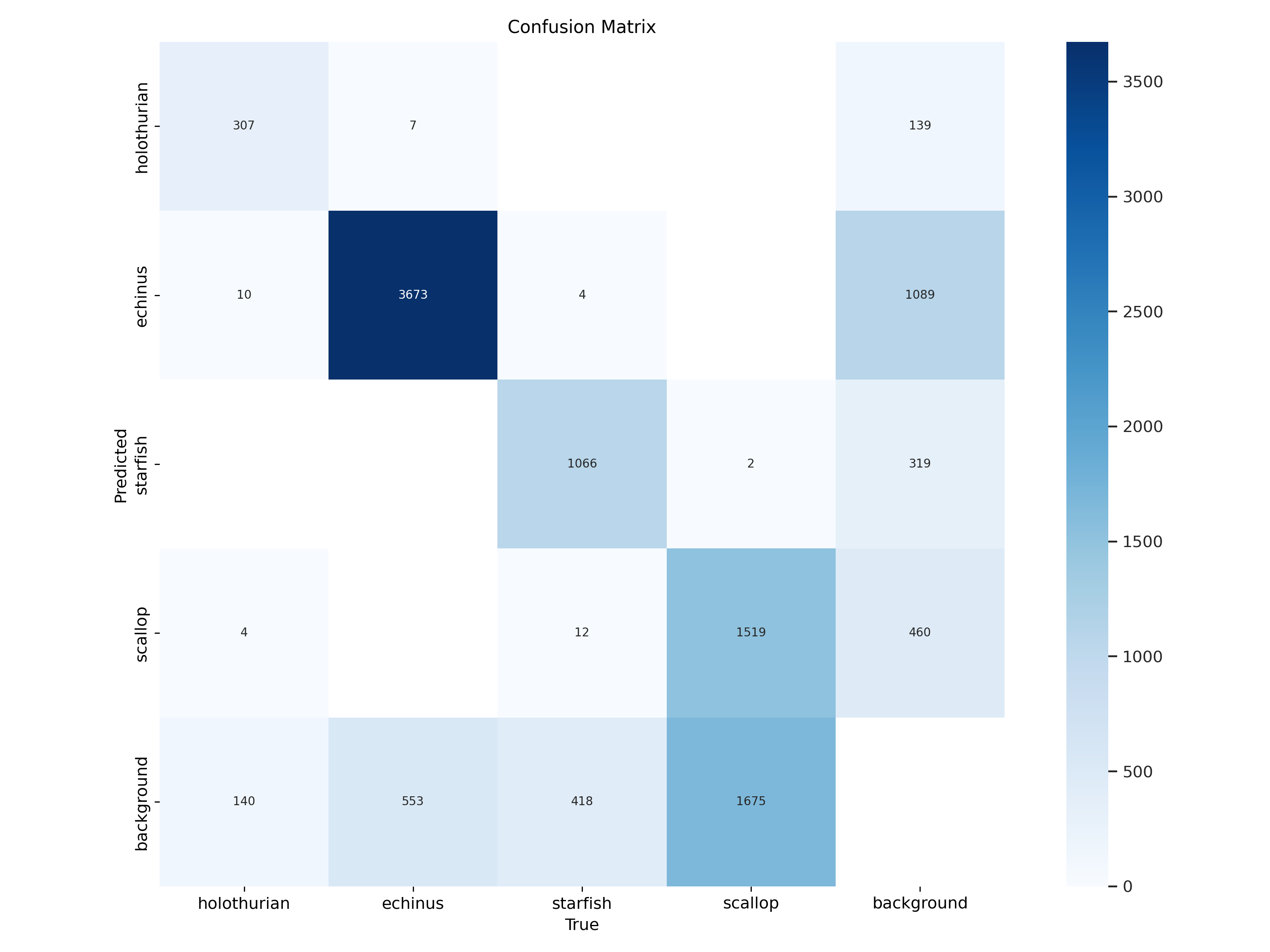
对于二分类问题，混淆矩阵通常是一个2×2的矩阵，包括真阳性（True Positive, TP）、真阴性（True Negative, TN）、假阳性（False Positive, FP）和假阴性（False Negative, FN）四个元素。

这个5*5的矩阵是这样理解的：

	真实值=holothurian	真实值=echinus	真实值=starfish	真实值=scallop	真实值=background
预测值=holothurian
预测值=echinus
预测值=starfish
预测值=scallop
预测值=background

而矩阵中的数值就是出现该情况的频次。

回到课程，为了方便程序编写，这节课的所有张量均放在CPU而非GPU上。回顾一下构建网络与训练网络：

python 复制代码

import torch
import torch.nn as nn
import torch.nn.functional as F
import torch.optim as optim  # short for optimizer. This can give us access to the optimizer we will use to update weights.

import torchvision
import torchvision.transforms as transforms


def get_num_correct(preds, labels):
    return preds.argmax(dim=1).eq(labels).sum().item()


torch.set_printoptions(linewidth=120)

train_set = torchvision.datasets.FashionMNIST(
    root='./data'
    , train=True
    , download=True
    , transform=transforms.Compose([
        transforms.ToTensor()
    ])
)


class Network(nn.Module):
    def __init__(self):
        super().__init__()
        self.conv1 = nn.Conv2d(in_channels=1, out_channels=6, kernel_size=5)
        self.conv2 = nn.Conv2d(in_channels=6, out_channels=12, kernel_size=5)
        self.fc1 = nn.Linear(in_features=12 * 4 * 4, out_features=120)
        self.fc2 = nn.Linear(in_features=120, out_features=60)
        self.out = nn.Linear(in_features=60, out_features=10)

    def forward(self, t):
        t = F.relu(self.conv1(t))
        t = F.max_pool2d(t, kernel_size=2, stride=2)
        t = F.relu(self.conv2(t))
        t = F.max_pool2d(t, kernel_size=2, stride=2)
        t = t.reshape(-1, 12 * 4 * 4)
        t = F.relu(self.fc1(t))
        t = F.relu(self.fc2(t))
        t = self.out(t)
        return t


network = Network()

train_loader = torch.utils.data.DataLoader(train_set, batch_size=100)    # step 1: Get batch from the training set.
optimizer = optim.Adam(network.parameters(), lr=0.005)


for epoch in range(5):
    total_loss = 0
    total_correct = 0

    for batch in train_loader:  # step 6: Repeat steps 1-5 until one epoch is completed.
        images, labels = batch

        preds = network(images) # step 2: Pass batch to network.
        loss = F.cross_entropy(preds, labels)   # step 3: Calculate the loss(difference between the predicted values and the true values).

        optimizer.zero_grad()
        loss.backward() # step 4: Calculate the gradient of the loss function w.r.t the network's weights.
        optimizer.step()    # step 5: Update the weights using the gradients to reduce the loss.

        total_loss += loss.item()
        total_correct += get_num_correct(preds, labels)

    print(f"epoch: {epoch}, average loss: {total_loss/len(train_loader):.10f}, average correct: {total_correct/len(train_loader):.10f}")

如果我们想要构建混淆矩阵，我们需要知道每一张图像的真实值、预测值，然后统计对应的次数，并绘制出图像。所以在训练完模型后，我们要用这个模型去预测：

python 复制代码

@torch.no_grad()
def get_all_preds(model, loader):
    all_preds = torch.tensor([])

    for batch in loader:
        images, labels = batch

        preds = model(images)
        all_preds = torch.cat((all_preds, preds), dim=0)

    return all_preds

prediction_loader = torch.utils.data.DataLoader(train_set, batch_size=10000)
train_preds = get_all_preds(network, prediction_loader)

print(f"train_set.targets.shape: {train_set.targets.shape}")
print(f"train_set.targets: {train_set.targets}")
print(f"train_preds.argmax(dim=1).shape: {train_preds.argmax(dim=1).shape}")
print(f"train_preds.argmax(dim=1): {train_preds.argmax(dim=1)}")

结果：

epoch: 0, average loss: 0.6142710297, average correct: 76.9300000000
epoch: 1, average loss: 0.4064236009, average correct: 85.1500000000
epoch: 2, average loss: 0.3550885973, average correct: 86.7516666667
epoch: 3, average loss: 0.3270902198, average correct: 87.8633333333
epoch: 4, average loss: 0.3086743477, average correct: 88.6150000000
train_set.targets.shape: 			torch.Size([60000])
train_set.targets: 					tensor([9, 0, 0,  ..., 3, 0, 5])
train_preds.argmax(dim=1).shape: 	torch.Size([60000])
train_preds.argmax(dim=1): 			tensor([9, 0, 0,  ..., 3, 0, 5])

可以看到刚刚的代码中有一段从来没见过的内容：@torch.no_grad()。关于这个语法，可以参考：【Python 高级特性】装饰器：不修改代码，就能改变函数功能的强大特性_哔哩哔哩_bilibili

关于关闭梯度，可以参考：28-CNN Confusion Matrix with PyTorch - Neural Network Programming_哔哩哔哩_bilibili，从08:30到12:46。

其中，train_set.targets就是所谓的真实值，train_preds.argmax(dim=1)就是所谓的预测值。如果预测值与真实值相等，说明预测正确；如果预测值与真实值不同，代表预测错误。

可以看到，train_set.targets和train_preds.argmax(dim=1)形状一样。现在我们把它们合并：

python 复制代码

stacked = torch.stack(
    (
        train_set.targets,
        train_preds.argmax(dim=1)
    ),
    dim=1
)

print(f"stacked.shape: {stacked.shape}")
print(f"stacked: {stacked}")

stacked.shape: 						torch.Size([60000, 2])
stacked: 							tensor([[9, 9],
                                            [0, 0],
                                            [0, 0],
                                            ...,
                                            [3, 3],
                                            [0, 0],
                                            [5, 5]])

从矩阵的角度理解，可以看作是先合并再进行转置。stacked左侧一列是真实值，右侧一列是预测值。由于我们是10分类，因此混淆矩阵应该是 10 × 10 10×10 10×10的，因此构建一个 10 × 10 10×10 10×10的张量：

python 复制代码

cmt = torch.zeros(10, 10, dtype=torch.int32)
print(cmt)

tensor([[0, 0, 0, 0, 0, 0, 0, 0, 0, 0],
        [0, 0, 0, 0, 0, 0, 0, 0, 0, 0],
        [0, 0, 0, 0, 0, 0, 0, 0, 0, 0],
        [0, 0, 0, 0, 0, 0, 0, 0, 0, 0],
        [0, 0, 0, 0, 0, 0, 0, 0, 0, 0],
        [0, 0, 0, 0, 0, 0, 0, 0, 0, 0],
        [0, 0, 0, 0, 0, 0, 0, 0, 0, 0],
        [0, 0, 0, 0, 0, 0, 0, 0, 0, 0],
        [0, 0, 0, 0, 0, 0, 0, 0, 0, 0],
        [0, 0, 0, 0, 0, 0, 0, 0, 0, 0]], dtype=torch.int32)

然后我们需要拆解stacked：

python 复制代码

for p in stacked:
    tl, pl = p.tolist() # true label & predict label
    cmt[tl, pl] = cmt[tl, pl] + 1

print(cmt)

其中，.tolist这个方法可以把某一个 1 × 2 1×2 1×2的张量拆分成两个数字。循环执行完60000次，就能拆分完stacked这个 60000 × 2 60000×2 60000×2的张量。结果如下：

tensor([[5111,    6,   32,  109,   15,    0,  670,    0,   57,    0],
        [   8, 5842,    3,  126,    3,    0,   12,    0,    6,    0],
        [  86,    1, 4084,   55,  856,    1,  826,    0,   91,    0],
        [ 159,   16,    7, 5495,  160,    0,  152,    0,   11,    0],
        [  13,    8,  160,  210, 4894,    0,  669,    0,   46,    0],
        [   1,    0,    0,    1,    0, 5651,    1,  187,   68,   91],
        [ 779,    7,  212,  108,  334,    1, 4464,    0,   95,    0],
        [   0,    0,    0,    0,    0,   17,    0, 5881,   26,   76],
        [  15,    1,    5,   19,   18,    1,   31,    2, 5908,    0],
        [   0,    0,    0,    0,    0,    7,    0,  323,    8, 5662]], dtype=torch.int32)

我们还可以把这个画成一张图，课程中给了个方法，也可以参考这篇博客：动手画混淆矩阵(Confusion Matrix)（含代码）_混淆矩阵怎么画-CSDN博客

把刚刚这篇博客中的代码移植过来：

python 复制代码

for p in stacked:
    tl, pl = p.tolist() # true label & predict label
    cmt[tl, pl] = cmt[tl, pl] + 1

print(cmt)

def draw_confusion_matrix(label_true, label_pred, label_name, title="Confusion Matrix", pdf_save_path=None, dpi=100):
    """

    @param label_true: 真实标签，比如[0,1,2,7,4,5,...]
    @param label_pred: 预测标签，比如[0,5,4,2,1,4,...]
    @param label_name: 标签名字，比如['cat','dog','flower',...]
    @param title: 图标题
    @param pdf_save_path: 是否保存，是则为保存路径pdf_save_path=xxx.png | xxx.pdf | ...等其他plt.savefig支持的保存格式
    @param dpi: 保存到文件的分辨率，论文一般要求至少300dpi
    @return:

    example：
            draw_confusion_matrix(label_true=y_gt,
                          label_pred=y_pred,
                          label_name=["Angry", "Disgust", "Fear", "Happy", "Sad", "Surprise", "Neutral"],
                          title="Confusion Matrix on Fer2013",
                          pdf_save_path="Confusion_Matrix_on_Fer2013.png",
                          dpi=300)

    """
    cm = confusion_matrix(y_true=label_true, y_pred=label_pred, normalize='true')

    plt.imshow(cm, cmap='Blues')
    plt.title(title)
    plt.xlabel("Predict label")
    plt.ylabel("Truth label")
    plt.yticks(range(label_name.__len__()), label_name)
    plt.xticks(range(label_name.__len__()), label_name, rotation=45)

    plt.tight_layout()

    plt.colorbar()

    for i in range(label_name.__len__()):
        for j in range(label_name.__len__()):
            color = (1, 1, 1) if i == j else (0, 0, 0)  # 对角线字体白色，其他黑色
            value = float(format('%.2f' % cm[j, i]))
            plt.text(i, j, value, verticalalignment='center', horizontalalignment='center', color=color)

    plt.show()
    if not pdf_save_path is None:
        plt.savefig(pdf_save_path, bbox_inches='tight', dpi=dpi)


draw_confusion_matrix(label_true=train_set.targets,
                      label_pred=train_preds.argmax(dim=1),
                      label_name=["T-shirt", "Trouser", "Pullover", "Dress", "Coat", "Sandal", "Shirt", "Sneaker", "Bag", "Ankle"],
                      title="Confusion Matrix on FashionMNIST",
                      pdf_save_path="D:\\Programme\\DeepLearning\\PyTorch\\test1\\Confusion_Matrix_on_FashionMNIST.jpg",
                      dpi=300)

需要额外import两个包：

python 复制代码

import matplotlib.pyplot as plt
from sklearn.metrics import confusion_matrix

在pip的时候需要注意，应该pip这个包：

pip install scikit-learn -i https://pypi.tuna.tsinghua.edu.cn/simple

来个10轮看看结果如何：

这节课就到此为止了，其实没啥东西，只是单纯造了个轮子。

3.4.Stack vs Concat - Deep Learning Tensor Ops

上节课有一段代码：

python 复制代码

stacked = torch.stack(
    (
        train_set.targets,
        train_preds.argmax(dim=1)
    ),
    dim=1
)

用的是Stack。这节课主要讲Stack和Concat的区别。

直接上结果吧：

python 复制代码

import torch

t1 = torch.tensor([1,1,1,1])
t2 = torch.tensor([2,2,2,2])
t3 = torch.tensor([3,3,3,3])

print(torch.cat((t1,t2,t3),dim=0))
# print(torch.cat((t1,t2,t3),dim=1))
# print(torch.cat((t1,t2,t3),dim=2))

print(torch.stack((t1,t2,t3),dim=0))
print(torch.stack((t1,t2,t3),dim=1))
# print(torch.stack((t1,t2,t3),dim=2))

其他几行注释掉是因为不符合语法。结果如下：

tensor([1, 1, 1, 1, 2, 2, 2, 2, 3, 3, 3, 3])
tensor([[1, 1, 1, 1],
        [2, 2, 2, 2],
        [3, 3, 3, 3]])
tensor([[1, 2, 3],
        [1, 2, 3],
        [1, 2, 3],
        [1, 2, 3]])

可见：

torch.cat((t1,t2,t3),dim=0)是直接横向拼接；
torch.stack((t1,t2,t3),dim=0)是换行拼接；
torch.stack((t1,t2,t3),dim=1)是先换行拼接再转置；

然后又讲了讲Tensorflow和Numpy中的操作，这里不再赘述。有兴趣的可以自己看一看：29-Stack vs Concat in PyTorch, TensorFlow & NumPy - Deep Learning Tensor Ops_哔哩哔哩_bilibili

3.5.Using TensorBoard with PyTorch - Analyzing Results Part 2

30-TensorBoard with PyTorch - Visualize Deep Learning Metrics_哔哩哔哩_bilibili

主要讲了TensorBoard这个工具的使用，暂时搁置一下。

3.6.Hyperparameter Experimenting - Training Neural Networks

和上一节课一样，还是讲TensorBoard这个工具。

4.Section 4: Neural Network Experimentation

如本章名字，这一章节是为了让我们自己建能够有效地试验我们所构建的训练过程。

4.1.Custom Code - Neural Network Experimentation Code

构建一个RunBuilder类，构建我们运行的参数集：

python 复制代码

class RunBuilder():
    @staticmethod
    def get_runs(params):
        Run = namedtuple('Run', params.keys())

        runs = []
        for v in product(*params.values()):
            runs.append(Run(*v))

        return runs

params = OrderedDict(lr = [.01,.005], batch_size = [100,500])

runs = RunBuilder.get_runs(params)
print(runs)

要添加如下import：

from collections import OrderedDict
from collections import namedtuple
from itertools import product

打印结果如下：

[Run(lr=0.01, batch_size=100), Run(lr=0.01, batch_size=500), Run(lr=0.005, batch_size=100), Run(lr=0.005, batch_size=500)]

也就是说，我们构建了4个不同的训练，分别为：

训练序号	learning rate	batch size
0	0.01	100
1	0.01	500
2	0.005	100
3	0.005	500

此外，还可以加别的参数，比如device，epoch等。并且，可以使用如下方法轻松打印出训练的信息：

python 复制代码

params = OrderedDict(lr = [.01,.005], batch_size = [100,500], device = ["cuda","cpu"], epoch = [100,200])

runs = RunBuilder.get_runs(params)
for run in RunBuilder.get_runs(params):
    comment = f'-{run}'
    print(comment)

-Run(lr=0.01, batch_size=100, device='cuda', epoch=100)
-Run(lr=0.01, batch_size=100, device='cuda', epoch=200)
-Run(lr=0.01, batch_size=100, device='cpu', epoch=100)
-Run(lr=0.01, batch_size=100, device='cpu', epoch=200)
-Run(lr=0.01, batch_size=500, device='cuda', epoch=100)
-Run(lr=0.01, batch_size=500, device='cuda', epoch=200)
-Run(lr=0.01, batch_size=500, device='cpu', epoch=100)
-Run(lr=0.01, batch_size=500, device='cpu', epoch=200)
-Run(lr=0.005, batch_size=100, device='cuda', epoch=100)
-Run(lr=0.005, batch_size=100, device='cuda', epoch=200)
-Run(lr=0.005, batch_size=100, device='cpu', epoch=100)
-Run(lr=0.005, batch_size=100, device='cpu', epoch=200)
-Run(lr=0.005, batch_size=500, device='cuda', epoch=100)
-Run(lr=0.005, batch_size=500, device='cuda', epoch=200)
-Run(lr=0.005, batch_size=500, device='cpu', epoch=100)
-Run(lr=0.005, batch_size=500, device='cpu', epoch=200)

4.2.Custom Code - Simultaneous Hyperparameter Testing

这节课主要讲了讲视频作者自己写的一个方法，目的是让训练部分的代码看起来更规整。而且代码在优化后，设置超参数可以更加清晰直观。如果有兴趣可以自己去看视频敲一遍代码，但是说实话视频里的方法过于复杂了，感觉意义不是很大。视频链接：33-CNN Training Loop Refactoring - Simultaneous Hyperparameter Testing_哔哩哔哩_bilibili

这里根据视频的思想，自己写了个精简版的：

python 复制代码

import torch
import torch.nn as nn
import torch.nn.functional as F
import torch.optim as optim  # short for optimizer. This can give us access to the optimizer we will use to update weights.

import torchvision
import torchvision.transforms as transforms

from collections import OrderedDict
from collections import namedtuple
from itertools import product


def get_num_correct(preds, labels):
    return preds.argmax(dim=1).eq(labels).sum().item()


class RunBuilder:
    @staticmethod
    def get_runs(params):
        Run = namedtuple('Run', params.keys())
        runs = []
        for v in product(*params.values()):
            runs.append(Run(*v))
        return runs


torch.set_printoptions(linewidth=120)

train_set = torchvision.datasets.FashionMNIST(
    root='./data'
    , train=True
    , download=True
    , transform=transforms.Compose([
        transforms.ToTensor()
    ])
)


class Network(nn.Module):
    def __init__(self):
        super().__init__()
        self.conv1 = nn.Conv2d(in_channels=1, out_channels=6, kernel_size=5)
        self.conv2 = nn.Conv2d(in_channels=6, out_channels=12, kernel_size=5)
        self.fc1 = nn.Linear(in_features=12 * 4 * 4, out_features=120)
        self.fc2 = nn.Linear(in_features=120, out_features=60)
        self.out = nn.Linear(in_features=60, out_features=10)

    def forward(self, t):
        t = F.relu(self.conv1(t))
        t = F.max_pool2d(t, kernel_size=2, stride=2)
        t = F.relu(self.conv2(t))
        t = F.max_pool2d(t, kernel_size=2, stride=2)
        t = t.reshape(-1, 12 * 4 * 4)
        t = F.relu(self.fc1(t))
        t = F.relu(self.fc2(t))
        t = self.out(t)
        return t


params = OrderedDict(
    lr=[.01, .005],
    batch_size=[100, 500],
    shuffle=[True, False],
    epoch=[5, 10],
    device=["cuda"]
)

for run in RunBuilder.get_runs(params):
    comment = f'-{run}'
    print(comment)

for run in RunBuilder.get_runs(params):
    comment = f'-{run}'
    print(f"\n\n")
    print(comment)

    network = Network()

    train_loader = torch.utils.data.DataLoader(train_set, batch_size=run.batch_size, shuffle=run.shuffle)  # step 1: Get batch from the training set.
    optimizer = optim.Adam(network.parameters(), lr=run.lr)

    device = run.device
    network.to(device)

    for epoch in range(run.epoch):
        total_loss = 0
        total_correct = 0

        for batch in train_loader:  # step 6: Repeat steps 1-5 until one epoch is completed.
            images, labels = batch
            images, labels = images.to(device), labels.to(device)

            preds = network(images)  # step 2: Pass batch to network.
            loss = F.cross_entropy(preds, labels)  # step 3: Calculate the loss(difference between the predicted values and the true values).

            optimizer.zero_grad()
            loss.backward()  # step 4: Calculate the gradient of the loss function w.r.t the network's weights.
            optimizer.step()  # step 5: Update the weights using the gradients to reduce the loss.

            total_loss += loss.item()
            total_correct += get_num_correct(preds, labels)

        print(f"epoch: {epoch}, average loss: {total_loss / len(train_loader):.10f}, average correct: {total_correct / len(train_loader):.10f}")

总共进行了16次训练，打印结果如下：

-Run(lr=0.01, batch_size=100, shuffle=True, epoch=5, device='cuda')
-Run(lr=0.01, batch_size=100, shuffle=True, epoch=10, device='cuda')
-Run(lr=0.01, batch_size=100, shuffle=False, epoch=5, device='cuda')
-Run(lr=0.01, batch_size=100, shuffle=False, epoch=10, device='cuda')
-Run(lr=0.01, batch_size=500, shuffle=True, epoch=5, device='cuda')
-Run(lr=0.01, batch_size=500, shuffle=True, epoch=10, device='cuda')
-Run(lr=0.01, batch_size=500, shuffle=False, epoch=5, device='cuda')
-Run(lr=0.01, batch_size=500, shuffle=False, epoch=10, device='cuda')
-Run(lr=0.005, batch_size=100, shuffle=True, epoch=5, device='cuda')
-Run(lr=0.005, batch_size=100, shuffle=True, epoch=10, device='cuda')
-Run(lr=0.005, batch_size=100, shuffle=False, epoch=5, device='cuda')
-Run(lr=0.005, batch_size=100, shuffle=False, epoch=10, device='cuda')
-Run(lr=0.005, batch_size=500, shuffle=True, epoch=5, device='cuda')
-Run(lr=0.005, batch_size=500, shuffle=True, epoch=10, device='cuda')
-Run(lr=0.005, batch_size=500, shuffle=False, epoch=5, device='cuda')
-Run(lr=0.005, batch_size=500, shuffle=False, epoch=10, device='cuda')



-Run(lr=0.01, batch_size=100, shuffle=True, epoch=5, device='cuda')
epoch: 0, average loss: 0.5920416600, average correct: 77.3633333333
epoch: 1, average loss: 0.4087048837, average correct: 84.6916666667
epoch: 2, average loss: 0.3676425663, average correct: 86.3216666667
epoch: 3, average loss: 0.3537376728, average correct: 86.8283333333
epoch: 4, average loss: 0.3422814391, average correct: 87.1783333333



-Run(lr=0.01, batch_size=100, shuffle=True, epoch=10, device='cuda')
epoch: 0, average loss: 0.5492223486, average correct: 79.1516666667
epoch: 1, average loss: 0.3799329826, average correct: 86.0050000000
epoch: 2, average loss: 0.3483632837, average correct: 87.2650000000
epoch: 3, average loss: 0.3277459771, average correct: 87.9200000000
epoch: 4, average loss: 0.3246190323, average correct: 88.0883333333
epoch: 5, average loss: 0.3123108984, average correct: 88.4750000000
epoch: 6, average loss: 0.3110108355, average correct: 88.7533333333
epoch: 7, average loss: 0.3071561582, average correct: 88.8133333333
epoch: 8, average loss: 0.2971438154, average correct: 88.9933333333
epoch: 9, average loss: 0.3020845860, average correct: 88.9533333333



-Run(lr=0.01, batch_size=100, shuffle=False, epoch=5, device='cuda')
epoch: 0, average loss: 0.5231307859, average correct: 80.5733333333
epoch: 1, average loss: 0.3721575903, average correct: 86.3266666667
epoch: 2, average loss: 0.3438053966, average correct: 87.2216666667
epoch: 3, average loss: 0.3264096088, average correct: 87.9566666667
epoch: 4, average loss: 0.3186341389, average correct: 88.1550000000



-Run(lr=0.01, batch_size=100, shuffle=False, epoch=10, device='cuda')
epoch: 0, average loss: 0.5866546286, average correct: 77.8483333333
epoch: 1, average loss: 0.3970952929, average correct: 85.3766666667
epoch: 2, average loss: 0.3621235035, average correct: 86.5833333333
epoch: 3, average loss: 0.3380681822, average correct: 87.5266666667
epoch: 4, average loss: 0.3294203746, average correct: 87.8300000000
epoch: 5, average loss: 0.3263481045, average correct: 87.8416666667
epoch: 6, average loss: 0.3185786353, average correct: 88.3183333333
epoch: 7, average loss: 0.3157054317, average correct: 88.3200000000
epoch: 8, average loss: 0.3133901746, average correct: 88.5316666667
epoch: 9, average loss: 0.3120996529, average correct: 88.5116666667



-Run(lr=0.01, batch_size=500, shuffle=True, epoch=5, device='cuda')
epoch: 0, average loss: 0.7892509239, average correct: 347.2750000000
epoch: 1, average loss: 0.4510333372, average correct: 416.3000000000
epoch: 2, average loss: 0.3713037593, average correct: 431.2583333333
epoch: 3, average loss: 0.3339587213, average correct: 437.6500000000
epoch: 4, average loss: 0.3173176558, average correct: 441.1083333333



-Run(lr=0.01, batch_size=500, shuffle=True, epoch=10, device='cuda')
epoch: 0, average loss: 0.7573039201, average correct: 354.0000000000
epoch: 1, average loss: 0.4501519705, average correct: 416.8416666667
epoch: 2, average loss: 0.3823612804, average correct: 429.3666666667
epoch: 3, average loss: 0.3457559437, average correct: 436.3666666667
epoch: 4, average loss: 0.3290857921, average correct: 438.6166666667
epoch: 5, average loss: 0.3094131328, average correct: 442.5833333333
epoch: 6, average loss: 0.2975341791, average correct: 444.1916666667
epoch: 7, average loss: 0.2881241533, average correct: 445.6333333333
epoch: 8, average loss: 0.2777063791, average correct: 447.7250000000
epoch: 9, average loss: 0.2732845400, average correct: 449.1750000000



-Run(lr=0.01, batch_size=500, shuffle=False, epoch=5, device='cuda')
epoch: 0, average loss: 0.7695579549, average correct: 353.5000000000
epoch: 1, average loss: 0.4608167340, average correct: 413.3000000000
epoch: 2, average loss: 0.3792866093, average correct: 429.6416666667
epoch: 3, average loss: 0.3401234890, average correct: 436.1416666667
epoch: 4, average loss: 0.3184403775, average correct: 439.4333333333



-Run(lr=0.01, batch_size=500, shuffle=False, epoch=10, device='cuda')
epoch: 0, average loss: 0.8925873876, average correct: 329.5416666667
epoch: 1, average loss: 0.4959731052, average correct: 408.4166666667
epoch: 2, average loss: 0.4143860998, average correct: 424.2666666667
epoch: 3, average loss: 0.3741927075, average correct: 431.2000000000
epoch: 4, average loss: 0.3524233627, average correct: 435.3083333333
epoch: 5, average loss: 0.3351472061, average correct: 437.7916666667
epoch: 6, average loss: 0.3246983716, average correct: 439.7833333333
epoch: 7, average loss: 0.3093644702, average correct: 442.6250000000
epoch: 8, average loss: 0.3039956290, average correct: 443.1333333333
epoch: 9, average loss: 0.2967160132, average correct: 444.8500000000



-Run(lr=0.005, batch_size=100, shuffle=True, epoch=5, device='cuda')
epoch: 0, average loss: 0.6199147650, average correct: 76.2400000000
epoch: 1, average loss: 0.3979324772, average correct: 85.2483333333
epoch: 2, average loss: 0.3547257959, average correct: 86.7416666667
epoch: 3, average loss: 0.3295163383, average correct: 87.7016666667
epoch: 4, average loss: 0.3138322780, average correct: 88.2683333333



-Run(lr=0.005, batch_size=100, shuffle=True, epoch=10, device='cuda')
epoch: 0, average loss: 0.6030920542, average correct: 77.0233333333
epoch: 1, average loss: 0.3808367471, average correct: 85.9150000000
epoch: 2, average loss: 0.3393732936, average correct: 87.4866666667
epoch: 3, average loss: 0.3147450837, average correct: 88.2833333333
epoch: 4, average loss: 0.3011448515, average correct: 88.7566666667
epoch: 5, average loss: 0.2857688793, average correct: 89.2666666667
epoch: 6, average loss: 0.2763760288, average correct: 89.6400000000
epoch: 7, average loss: 0.2677674725, average correct: 89.8633333333
epoch: 8, average loss: 0.2615216608, average correct: 90.0016666667
epoch: 9, average loss: 0.2529757225, average correct: 90.4666666667



-Run(lr=0.005, batch_size=100, shuffle=False, epoch=5, device='cuda')
epoch: 0, average loss: 0.6438212850, average correct: 75.6600000000
epoch: 1, average loss: 0.4311503610, average correct: 84.2750000000
epoch: 2, average loss: 0.3673974688, average correct: 86.3883333333
epoch: 3, average loss: 0.3370783451, average correct: 87.4566666667
epoch: 4, average loss: 0.3170995928, average correct: 88.1300000000



-Run(lr=0.005, batch_size=100, shuffle=False, epoch=10, device='cuda')
epoch: 0, average loss: 0.6074748931, average correct: 76.9666666667
epoch: 1, average loss: 0.3826813002, average correct: 85.7933333333
epoch: 2, average loss: 0.3360546749, average correct: 87.6816666667
epoch: 3, average loss: 0.3126871870, average correct: 88.4500000000
epoch: 4, average loss: 0.2962189508, average correct: 89.0433333333
epoch: 5, average loss: 0.2813491004, average correct: 89.4266666667
epoch: 6, average loss: 0.2728275024, average correct: 89.8183333333
epoch: 7, average loss: 0.2664490945, average correct: 89.9416666667
epoch: 8, average loss: 0.2537033156, average correct: 90.4100000000
epoch: 9, average loss: 0.2548490601, average correct: 90.4416666667



-Run(lr=0.005, batch_size=500, shuffle=True, epoch=5, device='cuda')
epoch: 0, average loss: 0.8625867729, average correct: 333.3500000000
epoch: 1, average loss: 0.5180763349, average correct: 403.0166666667
epoch: 2, average loss: 0.4419423719, average correct: 419.8916666667
epoch: 3, average loss: 0.3985803043, average correct: 427.3000000000
epoch: 4, average loss: 0.3671607743, average correct: 432.3166666667



-Run(lr=0.005, batch_size=500, shuffle=True, epoch=10, device='cuda')
epoch: 0, average loss: 0.8520629267, average correct: 340.1166666667
epoch: 1, average loss: 0.4742026764, average correct: 409.5500000000
epoch: 2, average loss: 0.3913912194, average correct: 427.4750000000
epoch: 3, average loss: 0.3563943662, average correct: 433.8916666667
epoch: 4, average loss: 0.3265873415, average correct: 439.5583333333
epoch: 5, average loss: 0.3126906040, average correct: 441.8333333333
epoch: 6, average loss: 0.2994723561, average correct: 444.2916666667
epoch: 7, average loss: 0.2842058177, average correct: 446.7250000000
epoch: 8, average loss: 0.2747114932, average correct: 448.5500000000
epoch: 9, average loss: 0.2636799593, average correct: 450.9416666667



-Run(lr=0.005, batch_size=500, shuffle=False, epoch=5, device='cuda')
epoch: 0, average loss: 0.8784389446, average correct: 333.3666666667
epoch: 1, average loss: 0.5245881908, average correct: 400.5166666667
epoch: 2, average loss: 0.4393276828, average correct: 420.1083333333
epoch: 3, average loss: 0.3916752331, average correct: 428.3000000000
epoch: 4, average loss: 0.3638193076, average correct: 432.9500000000



-Run(lr=0.005, batch_size=500, shuffle=False, epoch=10, device='cuda')
epoch: 0, average loss: 0.8776366348, average correct: 335.2666666667
epoch: 1, average loss: 0.5421455326, average correct: 397.2833333333
epoch: 2, average loss: 0.4568016176, average correct: 416.8500000000
epoch: 3, average loss: 0.4070300584, average correct: 426.6000000000
epoch: 4, average loss: 0.3699127187, average correct: 432.5750000000
epoch: 5, average loss: 0.3440336622, average correct: 436.9833333333
epoch: 6, average loss: 0.3256822807, average correct: 440.0166666667
epoch: 7, average loss: 0.3118922246, average correct: 442.4250000000
epoch: 8, average loss: 0.3020313072, average correct: 444.0000000000
epoch: 9, average loss: 0.2944910130, average correct: 445.3666666667

其实仔细观察代码，与我们3.2节写的并没有太大差别。用Git瞅一瞅：

其实真的差不多，仔细看看有差别的地方就能轻松理解。

视频里的那个方法看似高大上实际也确实高大上，但是本质还是这些操作，只不过加了很多代码来实现一些附加功能，比如打印结果更好看、用TensorBoard、计算时间等等。我是感觉暂时先不用管，这属于支线任务。

4.3.Data Loading - Deep Learning Speed Limit Increase

重头戏来了：如何加速神经网络。

有一个参数是num_workers ，这个参数用来决定有几个工人参与到训练任务中。修改代码如下：

python 复制代码

params = OrderedDict(
    lr=[.01],
    batch_size=[100],
    shuffle=[True],
    epoch=[5],
    device=["cuda"],
    num_workers=[0,1,2,4,8,16]
)


def main():
    for run in RunBuilder.get_runs(params):
        comment = f'-{run}'
        print(comment)

    for run in RunBuilder.get_runs(params):
        comment = f'-{run}'
        print(f"\n\n")
        print(comment)

        network = Network()

        train_loader = torch.utils.data.DataLoader(train_set, batch_size=run.batch_size, shuffle=run.shuffle, num_workers=run.num_workers)  # step 1: Get batch from the training set.
        optimizer = optim.Adam(network.parameters(), lr=run.lr)

        device = run.device
        network.to(device)

        train_start_time = time.time()
        for epoch in range(run.epoch):
            total_loss = 0
            total_correct = 0

            for batch in train_loader:  # step 6: Repeat steps 1-5 until one epoch is completed.
                images, labels = batch
                images, labels = images.to(device), labels.to(device)

                preds = network(images)  # step 2: Pass batch to network.
                loss = F.cross_entropy(preds, labels)  # step 3: Calculate the loss(difference between the predicted values and the true values).

                optimizer.zero_grad()
                loss.backward()  # step 4: Calculate the gradient of the loss function w.r.t the network's weights.
                optimizer.step()  # step 5: Update the weights using the gradients to reduce the loss.

                total_loss += loss.item()
                total_correct += get_num_correct(preds, labels)

            print(f"epoch: {epoch}, average loss: {total_loss / len(train_loader):.10f}, average correct: {total_correct / len(train_loader):.10f}")
        train_end_time = time.time()
        print(f"train time: {train_end_time - train_start_time:.10f}")


if __name__ == '__main__':
    main()

为了避免windows在多进程时出现错误，需要把多进程的逻辑放入main()方法中。此外，我还加了一个计算训练时间的小逻辑，需要额外import time。使用Git看一下差异：

结果如下：

-Run(lr=0.01, batch_size=100, shuffle=True, epoch=5, device='cuda', num_workers=0)
epoch: 0, average loss: 0.5889489330, average correct: 77.6366666667
epoch: 1, average loss: 0.3963580837, average correct: 85.3083333333
epoch: 2, average loss: 0.3774351805, average correct: 86.1550000000
epoch: 3, average loss: 0.3641082152, average correct: 86.5716666667
epoch: 4, average loss: 0.3537526523, average correct: 86.9150000000
train time: 25.0075454712



-Run(lr=0.01, batch_size=100, shuffle=True, epoch=5, device='cuda', num_workers=1)
epoch: 0, average loss: 0.5542732583, average correct: 78.9266666667
epoch: 1, average loss: 0.3714919458, average correct: 86.3066666667
epoch: 2, average loss: 0.3456784629, average correct: 87.3250000000
epoch: 3, average loss: 0.3339744434, average correct: 87.8033333333
epoch: 4, average loss: 0.3226663608, average correct: 88.0750000000
train time: 43.3679795265



-Run(lr=0.01, batch_size=100, shuffle=True, epoch=5, device='cuda', num_workers=2)
epoch: 0, average loss: 0.5282431153, average correct: 80.0533333333
epoch: 1, average loss: 0.3752922985, average correct: 85.9616666667
epoch: 2, average loss: 0.3499810995, average correct: 86.8783333333
epoch: 3, average loss: 0.3324256434, average correct: 87.7316666667
epoch: 4, average loss: 0.3266595144, average correct: 87.8866666667
train time: 39.0620391369



-Run(lr=0.01, batch_size=100, shuffle=True, epoch=5, device='cuda', num_workers=4)
epoch: 0, average loss: 0.5689649721, average correct: 78.4050000000
epoch: 1, average loss: 0.3926167285, average correct: 85.4866666667
epoch: 2, average loss: 0.3640779927, average correct: 86.4366666667
epoch: 3, average loss: 0.3475985242, average correct: 87.1316666667
epoch: 4, average loss: 0.3318750289, average correct: 87.7633333333
train time: 39.0912690163



-Run(lr=0.01, batch_size=100, shuffle=True, epoch=5, device='cuda', num_workers=8)
epoch: 0, average loss: 0.5755973245, average correct: 78.3383333333
epoch: 1, average loss: 0.3899452185, average correct: 85.6650000000
epoch: 2, average loss: 0.3616473807, average correct: 86.6100000000
epoch: 3, average loss: 0.3443661022, average correct: 87.1650000000
epoch: 4, average loss: 0.3380884284, average correct: 87.5900000000
train time: 48.0404033661



-Run(lr=0.01, batch_size=100, shuffle=True, epoch=5, device='cuda', num_workers=16)
epoch: 0, average loss: 0.5969337454, average correct: 77.3150000000
epoch: 1, average loss: 0.4035679932, average correct: 85.0200000000
epoch: 2, average loss: 0.3586135743, average correct: 86.8533333333
epoch: 3, average loss: 0.3403906616, average correct: 87.4583333333
epoch: 4, average loss: 0.3330876943, average correct: 87.8000000000
train time: 68.1281514168

可以看到，按训练速度排序，依次为num_workers=0, 2, 4, 1, 8, 16。这就很奇怪了，与课程完全不符。根据视频，理想情况下应该是num_workers=1时最快：一个worker在进行forward和backward的时候，另一个worker去加载数据，两个人如此往复应该效率非常高；如果num_workers=0，那一个人不如俩人并行干活快；如果num_workers多于1，那应该总有人闲着没事干。为什么会出现这个情况呢？

问了一下GPT：

CPU 和 GPU 资源竞争

在使用 num_workers > 0 时，PyTorch 使用了多进程来并行加载数据，这会增加 CPU 的负担。特别是在 GPU 和 CPU 资源有限的情况下，数据加载可能会成为瓶颈。

GPU 并行计算与 CPU 数据加载的竞争：虽然 GPU 可以加速计算，但在多线程/多进程加载数据时，CPU 会变得繁忙，特别是当数据预处理比较复杂或者 CPU 核心不够时。多个 worker 在处理数据时需要不断与主进程进行通信，从而增加了额外的开销。

IO瓶颈 ：如果你使用的是磁盘（而非 SSD）读取数据，IO 会成为瓶颈。当 num_workers 增加时，多个进程可能会同时进行磁盘访问，导致 IO 操作更加拥塞，从而导致性能下降。

过多的进程导致调度开销

当你使用多个 worker 时，PyTorch 会为每个 worker 创建一个进程来加载数据。每个进程都需要一些时间来启动并管理。增加 worker 数量的同时也意味着每个进程在进行通信、同步等操作时所需的开销会显著增加，导致性能变差。

进程管理和通信 ：在多进程模式下，每个 worker 之间需要进行数据传递和同步，特别是在 num_workers 较高时，Python 进程间的管理开销会增加。这个开销可能会抵消数据加载的加速效应。

Windows的multiprocessing问题 ：在 Windows 系统中，multiprocessing 会带来额外的开销。Python 需要在每个进程中重新导入模块，可能导致性能下降。

数据加载的速度与网络带宽限制

如果你的数据集较小或读取速度较快，当 num_workers 过高时，可能会有多余的进程在等待数据加载或过多的进程在闲置状态，导致 CPU 的过度切换和内存缓存溢出等问题。

内存带宽或缓存问题

使用多个 worker 时，数据的加载和处理可能会频繁占用内存，特别是当数据集非常大时。内存带宽可能成为瓶颈，导致缓存失效和数据的等待，最终拖慢整体的训练速度。

于是我关闭了除Pycharm之外的所有程序，并且测试了device="cpu"的情况：

把结果整理成表格，如下所示：

Device	num_workers=0	num_workers=1	num_workers=2	num_workers=4	num_workers=8	num_workers=16
CPU	22.7454195023	38.8810143471	39.3634419441	39.1821424961	50.9369196892	66.9246480465
GPU	21.2091612816	37.8195934296	33.8372309208	33.2044763565	41.2324335575	55.7895495892

这一次按训练速度排序，依次为num_workers=0, 4, 2, 1, 8, 16。说明GPT多半在胡扯，这下完全解释不通了。

用于对照，我又租了云服务器，看看用满血RTX 4090(24GB)训练的结果如何。为了节省时间，只测试GPU，结果如下：

Device	num_workers=0	num_workers=1	num_workers=2	num_workers=4	num_workers=8	num_workers=16
GPU	19.8094530106	18.6171827316	10.8715770245	10.2341358662	11.0814673901	12.2236852646

按训练速度排序，依次为num_workers=4, 2, 8, 16, 1, 0。这既不是视频预测的顺序，也不是刚刚在本地实测的顺序，又不是升序，又不是降序，让我很难办啊...

那调整一下别的超参数试试：

dv	lr	bs	ep	num=0	num=1	num=2	num=4	num=8	num=16
GPU	0.01	100	5	19.8094530106	18.6171827316	10.8715770245	10.2341358662	11.0814673901	12.2236852646
GPU	0.01	100	10	39.1413171291	37.4858777523	22.0164945126	20.8994820118	22.1796212196	23.8738613129
GPU	0.01	100	15	57.7995896339	54.7732126713	31.0987980366	30.4089231491	32.7723743916	35.4690580368
GPU	0.01	100	20	77.1752855778	75.3958535194	41.2066097260	41.6991536617	44.0119616985	48.2091443539
GPU	0.01	200	5	16.7913942337	16.7396118641	9.9124171734	5.8958966732	5.9714968204	7.0907850266
GPU	0.01	200	10	31.5285310745	34.1176443100	18.5157856941	11.9089007378	12.8334674835	14.0546066761
GPU	0.01	200	15	47.4661595821	51.3070929050	27.9936087132	17.6425700188	19.1162984371	22.1769638062
GPU	0.01	200	20	64.2943732738	67.6741607189	38.3087828159	23.1501190662	26.6771740913	38.7755141258

其中，dv是Device，lr是learning rate，bs是batch size，ep是epoch，num都指num_workers。

先不管本地，看一看云服务器。虽然既不是升序又不是降序，但是很明显，除了在learning rate=0.01、batch size=100、epoch=20这个条件下之外，其他的几次训练都是在num_workers=4之前时间依次递减，在num_workers=4之后时间一次递增。虽然不清楚原因，但是现象确实是这样的。如果有读者能够指出这种现象的原因，笔者不胜感激。

在此，我先后有两个猜想，不过经过对照实验均已证伪。这里只是放一下，完全可以不看。猜想1：有没有可能是对服务器而言，读取learn_loader的速度远远慢于训练5个epoch的速度，且这个速度大约差4倍。如果有num_workers=4，即，以类似5级（4+1）流水线的方式工作，恰好满足4个工人读取learn_loader，1个工人进行forward和backward，此时工作效率最高；如果num_workers<4，则此时活干不完；如果num_workers>4，则此时有工人总闲着没事干。但是我回看了代码，想起测量的这个时间本身就不包含读取learn_loader，所以肯定不对。不过我也实测了一下，不论是本地还是服务器，读取learn_loader的时间均在1ms以内，完全不存在读取learn_loader耗费很多时间的可能。猜想2：会不会在num_workers<4的时候，没有完全利用完GPU的资源；在num_workers>4的时候，GPU的资源已经被利用到100%，所以会随着num_workers的增加，运行负担越来越高，从而导致训练时间越来越长。为了验证，我们将learning rate设置为0.01，batch size设置为100，epoch设置为5，只改变num_workers的值。同时，在服务器中打开AutoPanel，监控GPU的使用率。然而发现，不论是GPU、CPU、显存、内存都没有跑满，甚至冗余很多。非常之奇怪啊。

不过这个东西似乎也不用斤斤计较，因为num_workers的设置只影响训练需要浪费掉的时间，并不会影响我们的训练结果。真正影响网络性能的还是网络结构和权重，因此这个问题就暂时搁置吧。

附一下我做的其他测试，其中，RTX 4090(24GB)、RTX 3090(24GB)代表在云服务器进行的测试，RTX 4070(16GB) Laptop代表在本地进行的测试：

dv	lr	bs	ep	num=0	num=1	num=2	num=4	num=8	num=16
RTX 4070(16GB) Laptop	0.01	100	5	28.1305768490	41.7332050800	36.2673246861	34.3168334961	39.9641251564	57.6469037533
RTX 4070(16GB) Laptop	0.01	100	10	57.8800597191	81.7754955292	73.1815102100	65.6602911949	77.4903655052	118.0588462353
RTX 4070(16GB) Laptop	0.01	100	15	99.5685005188	130.0420460701	111.5567693710	107.4449329376	132.9369020462	182.7950754166
RTX 4070(16GB) Laptop	0.01	100	20	141.9266636372	170.4486801624	159.7556915283	146.8164608479	172.9068100452	230.8282351494
RTX 3090(24GB)	0.01	100	5	29.5825061798	26.8633742332	17.8401007652	19.9198176861	19.0827801228	21.7736520767
RTX 3090(24GB)	0.01	100	10	58.3652188778	53.4312276840	36.3988366127	35.5191409588	36.3807988167	38.4931862354
RTX 3090(24GB)	0.01	100	15	88.5150232315	79.5371186733	59.6383686066	53.8375451565	54.5288057327	63.0430862904
RTX 3090(24GB)	0.01	100	20	117.6886110306	105.9683313370	83.1662738323	83.4657490253	83.4540984631	87.3529927731
RTX 3090(24GB)	0.01	200	5	25.3283810616	24.0916061401	13.5204551220	12.0049178600	11.2450921535	12.2135033607
RTX 3090(24GB)	0.01	200	10	48.6335105896	48.8655605316	26.1286144257	21.2161135674	21.9887542725	23.7948474884
RTX 3090(24GB)	0.01	200	15	72.6389396191	73.0067055225	38.1936340332	33.8487656116	30.4887382984	33.7346482277
RTX 3090(24GB)	0.01	200	20	97.3576982021	96.1663630009	54.2182519436	43.7375555038	43.9286410809	50.3938348293
RTX 4090(24GB)	0.01	100	5	19.8094530106	18.6171827316	10.8715770245	10.2341358662	11.0814673901	12.2236852646
RTX 4090(24GB)	0.01	100	10	39.1413171291	37.4858777523	22.0164945126	20.8994820118	22.1796212196	23.8738613129
RTX 4090(24GB)	0.01	100	15	57.7995896339	54.7732126713	31.0987980366	30.4089231491	32.7723743916	35.4690580368
RTX 4090(24GB)	0.01	100	20	77.1752855778	75.3958535194	41.2066097260	41.6991536617	44.0119616985	48.2091443539
RTX 4090(24GB)	0.01	200	5	16.7913942337	16.7396118641	9.9124171734	5.8958966732	5.9714968204	7.0907850266
RTX 4090(24GB)	0.01	200	10	31.5285310745	34.1176443100	18.5157856941	11.9089007378	12.8334674835	14.0546066761
RTX 4090(24GB)	0.01	200	15	47.4661595821	51.3070929050	27.9936087132	17.6425700188	19.1162984371	22.1769638062
RTX 4090(24GB)	0.01	200	20	64.2943732738	67.6741607189	38.3087828159	23.1501190662	26.6771740913	38.7755141258
RTX 4090(24GB)	0.01	100	100	394.7647271156	390.7899484634	218.7683389187	212.3276288509	221.9496636391	242.6673545837
RTX 4090(24GB)	0.01	100	150	552.9656944275	536.8140552044	308.1492588520	312.5498087406	330.0487678051	375.0175244808
RTX 4090(24GB)	0.01	100	200	739.6282594204	733.0374395847	405.3113956451	418.5048103333	437.4574213028	477.0259277821
RTX 4090(24GB)	0.01	200	100	338.4314348698	359.8767967224	199.4675915241	121.1487936974	136.2409780025	173.8709726334
RTX 4090(24GB)	0.01	200	150	472.6995038986	499.8453207016	282.8549370766	189.5168559551	200.7765417099	236.5929512978
RTX 4090(24GB)	0.01	200	200	675.4776511192	721.8856656551	395.7786476612	243.3258059025	263.1972572803	310.2211456299

4.4.On the GPU - Training Neural Networks with CUDA

没什么新东西，之前我就已经把网络和张量放到GPU上了。

4.5.Data Normalization - Normalize a Dataset

这节课的目标是将原始数据集标准化，并对比标准化后的数据集和原始数据集。

注意：本节课中代码涉及到num_workers的设置，如果是在windows上运行需要删掉，或者把这一部分放到main函数中！

首先和之前一样，获取一下数据集：

python 复制代码

import torch

import torchvision
import torchvision.transforms as transforms

import matplotlib.pyplot as plt


train_set = torchvision.datasets.FashionMNIST(
    root='./data'
    , train=True
    , download=True
    , transform=transforms.Compose([
        transforms.ToTensor()
    ])
)

有两种方法可以求平均值和标准差：

python 复制代码

# Easy way: Calculate the mean and standard deviation using the torch method
loader = torch.utils.data.DataLoader(train_set, batch_size=len(train_set), num_workers=4)
data = next(iter(loader))
print(data[0].mean(), data[0].std())


# Harder way: Calculate the mean and standard deviation by hands
loader = torch.utils.data.DataLoader(train_set, batch_size=len(train_set), num_workers=4)
num_of_pixels = len(train_set) * 28 * 28

total_sum = 0
for batch in loader:
    total_sum += batch[0].sum()
mean = total_sum / num_of_pixels

sum_of_squared_error = 0
for batch in loader:
    sum_of_squared_error += ((batch[0] - mean) ** 2).sum()
std = torch.sqrt(sum_of_squared_error / num_of_pixels)

print(mean, std)

注意：这里设置了num_workers=4，如果是在windows上运行需要删掉这一部分，或者把这一部分放到main函数中！在代码的其他部分同样也要注意这个问题，不再反复提示！

运行的结果是一样的：

tensor(0.2860) tensor(0.3530)
tensor(0.2860) tensor(0.3530)

直接用简单的那个方法就行。需要注意的是这段代码非常吃内存，因为一下子加载了60000张图片。然后画一个直方图，把我们的data[0]展开：

python 复制代码

plt.hist(data[0].flatten())
plt.axvline(data[0].mean())
plt.show()

需要注意data[0]的大小，这是一个60000*1*28*28的张量。横坐标表示具体的值（由于FashionMNIST数据集是灰度图，所以每一个value都在0-1之间），纵坐标表示个数（ × 1 0 7 ×10^7 ×107），竖线是平均值。

然后我们标准化一下，看看会发生什么样的变化：

python 复制代码

train_set_normal = torchvision.datasets.FashionMNIST(
    root='./data'
    , train=True
    , download=True
    , transform=transforms.Compose([
        transforms.ToTensor(),
        # normalize
        transforms.Normalize(data[0].mean(), data[0].std())
    ])
)

# Easy way: Calculate the mean and standard deviation using the torch method
loader_normal = torch.utils.data.DataLoader(train_set_normal, batch_size=len(train_set_normal), num_workers=4)
data_normal = next(iter(loader_normal))
print(data_normal[0].mean(), data_normal[0].std())

plt.hist(data_normal[0].flatten())
plt.axvline(data_normal[0].mean())
plt.show()

结果如下：

tensor(0.2860) tensor(0.3530)
tensor(-2.9064e-08) tensor(1.)

对比一下代码：

经过标准化后，均值约为0，标准差约为1，这就是标准化操作带来的影响。

为什么要费这么大劲对数据进行标准化呢？我们分别训练一下，先看一看完整代码：

python 复制代码

import time

import torch
import torch.nn as nn
import torch.nn.functional as F
import torch.optim as optim  # short for optimizer. This can give us access to the optimizer we will use to update weights.

import torchvision
import torchvision.transforms as transforms

from collections import OrderedDict
from collections import namedtuple
from itertools import product


def get_num_correct(preds, labels):
    return preds.argmax(dim=1).eq(labels).sum().item()


class RunBuilder:
    @staticmethod
    def get_runs(params):
        Run = namedtuple('Run', params.keys())
        runs = []
        for v in product(*params.values()):
            runs.append(Run(*v))
        return runs


torch.set_printoptions(linewidth=120)

train_set_not_normal = torchvision.datasets.FashionMNIST(
    root='./data'
    , train=True
    , download=True
    , transform=transforms.Compose([
        transforms.ToTensor()
        # normalize

    ])
)

# Easy way: Calculate the mean and standard deviation using the torch method
loader = torch.utils.data.DataLoader(train_set_not_normal, batch_size=len(train_set_not_normal), num_workers=4)
data = next(iter(loader))

train_set_normal = torchvision.datasets.FashionMNIST(
    root='./data'
    , train=True
    , download=True
    , transform=transforms.Compose([
        transforms.ToTensor(),
        # normalize
        transforms.Normalize((data[0].mean()), (data[0].std()))
    ])
)

# Easy way: Calculate the mean and standard deviation using the torch method
loader_normal = torch.utils.data.DataLoader(train_set_normal, batch_size=len(train_set_normal), num_workers=4)
data_normal = next(iter(loader_normal))


class Network(nn.Module):
    def __init__(self):
        super().__init__()
        self.conv1 = nn.Conv2d(in_channels=1, out_channels=6, kernel_size=5)
        self.conv2 = nn.Conv2d(in_channels=6, out_channels=12, kernel_size=5)
        self.fc1 = nn.Linear(in_features=12 * 4 * 4, out_features=120)
        self.fc2 = nn.Linear(in_features=120, out_features=60)
        self.out = nn.Linear(in_features=60, out_features=10)

    def forward(self, t):
        t = F.relu(self.conv1(t))
        t = F.max_pool2d(t, kernel_size=2, stride=2)
        t = F.relu(self.conv2(t))
        t = F.max_pool2d(t, kernel_size=2, stride=2)
        t = t.reshape(-1, 12 * 4 * 4)
        t = F.relu(self.fc1(t))
        t = F.relu(self.fc2(t))
        t = self.out(t)
        return t


params = OrderedDict(
    train_set=[train_set_not_normal, train_set_normal],
    lr=[.01],
    batch_size=[100],
    shuffle=[True],
    epoch=[100],
    num_workers=[4],
    device=["cuda"]
)


def main():
    for run in RunBuilder.get_runs(params):
        comment = f'-{run}'
        print(comment)

    for run in RunBuilder.get_runs(params):
        comment = f'-{run}'
        print(f"\n")
        print(comment)

        network = Network()

        reading_start_time = time.time()
        train_loader = torch.utils.data.DataLoader(dataset=run.train_set,
                                                   batch_size=run.batch_size,
                                                   shuffle=run.shuffle,
                                                   num_workers=run.num_workers)  # step 1: Get batch from the training set.
        optimizer = optim.Adam(network.parameters(), lr=run.lr)

        device = run.device
        network.to(device)
        reading_end_time = time.time()
        # print(f"reading train loader time: {reading_end_time - reading_start_time:.10f}")

        train_start_time = time.time()
        for epoch in range(run.epoch):  # step 7: Repeat steps 1-6 for as many epochs required to obtain the desired level of accuracy.
            total_loss = 0
            total_correct = 0

            for batch in train_loader:  # step 6: Repeat steps 1-5 until one epoch is completed.
                images, labels = batch
                images, labels = images.to(device), labels.to(device)

                preds = network(images)  # step 2: Pass batch to network.
                loss = F.cross_entropy(preds, labels)  # step 3: Calculate the loss(difference between the predicted values and the true values).

                optimizer.zero_grad()
                loss.backward()  # step 4: Calculate the gradient of the loss function w.r.t the network's weights.
                optimizer.step()  # step 5: Update the weights using the gradients to reduce the loss.

                total_loss += loss.item()
                total_correct += get_num_correct(preds, labels)

            print(
                f"epoch: {epoch}, average loss: {total_loss / len(train_loader):.10f}, average correct: {total_correct / len(train_loader):.10f}")
        train_end_time = time.time()
        print(f"train time: {train_end_time - train_start_time:.10f}")


if __name__ == '__main__':
    main()

老样子，用Git看差异：

应该很简单易懂吧。这里我把num_workers设成了4，虽然不知道为什么这样最快，但是实测这样确实最快（雾）。

偷偷加了一个排序，直接把main换了就行，有兴趣就自己看看代码区别：

python 复制代码

def main():
    # for run in RunBuilder.get_runs(params):
    #     comment = f'-{run}'
    #     print(comment)

    results = []

    for run in RunBuilder.get_runs(params):
        comment = f'-{run}'
        print(f"\n")
        print(comment)

        network = Network()

        reading_start_time = time.time()
        train_loader = torch.utils.data.DataLoader(dataset=run.train_set,
                                                   batch_size=run.batch_size,
                                                   shuffle=run.shuffle,
                                                   num_workers=run.num_workers)  # step 1: Get batch from the training set.
        optimizer = optim.Adam(network.parameters(), lr=run.lr)

        device = run.device
        network.to(device)
        reading_end_time = time.time()
        # print(f"reading train loader time: {reading_end_time - reading_start_time:.10f}")

        train_start_time = time.time()
        for epoch in range(run.epoch):  # step 7: Repeat steps 1-6 for as many epochs required to obtain the desired level of accuracy.
            total_loss = 0
            total_correct = 0

            for batch in train_loader:  # step 6: Repeat steps 1-5 until one epoch is completed.
                images, labels = batch
                images, labels = images.to(device), labels.to(device)

                preds = network(images)  # step 2: Pass batch to network.
                loss = F.cross_entropy(preds, labels)  # step 3: Calculate the loss(difference between the predicted values and the true values).

                optimizer.zero_grad()
                loss.backward()  # step 4: Calculate the gradient of the loss function w.r.t the network's weights.
                optimizer.step()  # step 5: Update the weights using the gradients to reduce the loss.

                total_loss += loss.item()
                total_correct += get_num_correct(preds, labels)

            print(f"epoch: {epoch:3d}, average loss: {total_loss / len(train_loader):.10f}, average correct: {total_correct / len(train_loader):.10f}")

            results.append({
                'epoch': epoch,
                'average_loss': (total_loss / len(train_loader)),
                'average_correct': (total_correct / len(train_loader)),
                'train_set': 'not normal' if run.train_set == train_set_not_normal else 'normal'
            })

        train_end_time = time.time()
        # print(f"train time: {train_end_time - train_start_time:.10f}")

    sorted_results = sorted(results, key=lambda x: x['average_correct'], reverse=True)

    print("\nSorted Results (by average correct):")
    for result in sorted_results:
        print(f"epoch: {result['epoch']}, average loss: {result['average_loss']:.10f}, average correct: {result['average_correct']:.10f}, train_set: {result['train_set']}")

排序结果如下：

Sorted Results (by average correct):
epoch:  89, average loss: 0.2444642815, average correct: 91.3700000000, train_set: not normal
epoch:  94, average loss: 0.2436240145, average correct: 91.3250000000, train_set: not normal
epoch:  86, average loss: 0.2446894638, average correct: 91.2366666667, train_set: not normal
epoch:  95, average loss: 0.2503509281, average correct: 91.1933333333, train_set: not normal
epoch:  98, average loss: 0.2522871471, average correct: 91.1616666667, train_set: not normal
epoch:  93, average loss: 0.2487666017, average correct: 91.1300000000, train_set: not normal
epoch:  60, average loss: 0.2588673048, average correct: 91.0916666667, train_set: normal
epoch:  96, average loss: 0.2566552062, average correct: 91.0883333333, train_set: not normal
epoch:  88, average loss: 0.2468521763, average correct: 91.0700000000, train_set: not normal
epoch:  83, average loss: 0.2509987283, average correct: 91.0316666667, train_set: not normal
epoch:  92, average loss: 0.2598962237, average correct: 90.9683333333, train_set: not normal
epoch:  81, average loss: 0.2532719481, average correct: 90.9550000000, train_set: not normal
epoch:  70, average loss: 0.2449382489, average correct: 90.9533333333, train_set: not normal
epoch:  87, average loss: 0.2578270657, average correct: 90.9316666667, train_set: not normal
epoch:  90, average loss: 0.2609930170, average correct: 90.8933333333, train_set: not normal
epoch:  69, average loss: 0.2517988028, average correct: 90.8916666667, train_set: not normal
epoch:  67, average loss: 0.2641334045, average correct: 90.8883333333, train_set: normal
epoch:  59, average loss: 0.2651573863, average correct: 90.8733333333, train_set: normal
epoch:  76, average loss: 0.2493317663, average correct: 90.8700000000, train_set: not normal
epoch:  99, average loss: 0.2645902622, average correct: 90.8566666667, train_set: not normal
epoch:  82, average loss: 0.2623617617, average correct: 90.8383333333, train_set: not normal
epoch:  97, average loss: 0.2615160028, average correct: 90.8366666667, train_set: not normal
......

看样子是白忙活了，起码在learning rate=0.01，batch size=100，epoch=100时，使用原始数据集训练出来的效果更好，与原视频的结论正好相反。不过原视频中也提到对于不同的原始数据集、不同的网络结构、不同的超参数，使用标准化的数据集的训练效果和使用原始数据集的训练效果不一定哪个更好，需要具体实验才能得知。

不过我们搞都搞了，服务器也租了，那就再来一次，广泛实验。设置参数如下：

python 复制代码

params = OrderedDict(
    train_set=[train_set_not_normal, train_set_normal],
    lr=[.01,.005],
    batch_size=[100,200],
    shuffle=[True],
    epoch=[200],
    num_workers=[4],
    device=["cuda"]
)

然后把average correct这个参数换成了accuracy，main函数如下：

python 复制代码

def main():
    # for run in RunBuilder.get_runs(params):
    #     comment = f'-{run}'
    #     print(comment)

    results = []

    for run in RunBuilder.get_runs(params):
        comment = f'-{run}'
        print(f"\n")
        print(comment)

        network = Network()

        reading_start_time = time.time()
        train_loader = torch.utils.data.DataLoader(dataset=run.train_set,
                                                   batch_size=run.batch_size,
                                                   shuffle=run.shuffle,
                                                   num_workers=run.num_workers)  # step 1: Get batch from the training set.
        optimizer = optim.Adam(network.parameters(), lr=run.lr)

        device = run.device
        network.to(device)
        reading_end_time = time.time()
        # print(f"reading train loader time: {reading_end_time - reading_start_time:.10f}")

        train_start_time = time.time()
        for epoch in range(run.epoch):  # step 7: Repeat steps 1-6 for as many epochs required to obtain the desired level of accuracy.
            total_loss = 0
            total_correct = 0

            for batch in train_loader:  # step 6: Repeat steps 1-5 until one epoch is completed.
                images, labels = batch
                images, labels = images.to(device), labels.to(device)

                preds = network(images)  # step 2: Pass batch to network.
                loss = F.cross_entropy(preds, labels)  # step 3: Calculate the loss(difference between the predicted values and the true values).

                optimizer.zero_grad()
                loss.backward()  # step 4: Calculate the gradient of the loss function w.r.t the network's weights.
                optimizer.step()  # step 5: Update the weights using the gradients to reduce the loss.

                total_loss += loss.item()
                total_correct += get_num_correct(preds, labels)

            print(f"epoch: {epoch:3d}, average loss: {total_loss / len(train_loader):.10f}, average correct: {total_correct / len(train_loader):.10f}")

            results.append({
                'epoch': epoch,
                'lr': run.lr,
                'batch_size': run.batch_size,
                'average_loss': (total_loss / len(train_loader)),
                'accuracy': (total_correct / len(train_loader) / run.batch_size),
                'train_set': 'not normal' if run.train_set == train_set_not_normal else 'normal'
            })

        train_end_time = time.time()
        print(f"train time: {train_end_time - train_start_time:.10f}")

    sorted_results = sorted(results, key=lambda x: x['accuracy'], reverse=True)

    print("\nSorted Results (by average correct):")
    for result in sorted_results:
        print(f"epoch: {result['epoch']:3d}, learning rate: {result['lr']:.3f}, batch size: {result['batch_size']}, average loss: {result['average_loss']:.10f}, accuracy: {result['accuracy']:.4f}, train_set: {result['train_set']}")

根据我们之前的测试，这一些全训练完大概要40分钟。经过漫长的等待，结果如下：

Sorted Results (by average correct):
epoch: 174, learning rate: 0.005, batch size: 200, average loss: 0.0709776129, accuracy: 0.9743, train_set: not normal
epoch: 193, learning rate: 0.005, batch size: 200, average loss: 0.0774264681, accuracy: 0.9724, train_set: not normal
epoch: 192, learning rate: 0.005, batch size: 200, average loss: 0.0803019308, accuracy: 0.9714, train_set: not normal
epoch: 189, learning rate: 0.005, batch size: 200, average loss: 0.0776055988, accuracy: 0.9713, train_set: not normal
epoch: 184, learning rate: 0.005, batch size: 200, average loss: 0.0794412048, accuracy: 0.9712, train_set: not normal
epoch: 184, learning rate: 0.005, batch size: 200, average loss: 0.0787860808, accuracy: 0.9711, train_set: normal
epoch: 180, learning rate: 0.005, batch size: 200, average loss: 0.0827256603, accuracy: 0.9709, train_set: not normal
epoch: 199, learning rate: 0.005, batch size: 200, average loss: 0.0837867468, accuracy: 0.9709, train_set: normal
epoch: 178, learning rate: 0.005, batch size: 200, average loss: 0.0792716932, accuracy: 0.9707, train_set: not normal
epoch: 188, learning rate: 0.005, batch size: 200, average loss: 0.0819608879, accuracy: 0.9707, train_set: not normal
epoch: 182, learning rate: 0.005, batch size: 200, average loss: 0.0838116156, accuracy: 0.9705, train_set: not normal
epoch: 155, learning rate: 0.005, batch size: 200, average loss: 0.0803890361, accuracy: 0.9704, train_set: not normal
epoch: 176, learning rate: 0.005, batch size: 200, average loss: 0.0855941821, accuracy: 0.9699, train_set: normal
epoch: 169, learning rate: 0.005, batch size: 200, average loss: 0.0840451158, accuracy: 0.9699, train_set: not normal
epoch: 181, learning rate: 0.005, batch size: 200, average loss: 0.0859571979, accuracy: 0.9699, train_set: normal
epoch: 197, learning rate: 0.005, batch size: 200, average loss: 0.0866671357, accuracy: 0.9698, train_set: not normal
epoch: 162, learning rate: 0.005, batch size: 200, average loss: 0.0801894657, accuracy: 0.9698, train_set: not normal
epoch: 170, learning rate: 0.005, batch size: 200, average loss: 0.0910011409, accuracy: 0.9695, train_set: normal
epoch: 189, learning rate: 0.005, batch size: 200, average loss: 0.0871327942, accuracy: 0.9695, train_set: normal
epoch: 183, learning rate: 0.005, batch size: 200, average loss: 0.0858964958, accuracy: 0.9694, train_set: not normal
epoch: 177, learning rate: 0.005, batch size: 200, average loss: 0.0875864697, accuracy: 0.9692, train_set: not normal
epoch: 185, learning rate: 0.005, batch size: 200, average loss: 0.0897819514, accuracy: 0.9691, train_set: normal
epoch: 194, learning rate: 0.005, batch size: 200, average loss: 0.0898394302, accuracy: 0.9690, train_set: normal
epoch: 152, learning rate: 0.005, batch size: 200, average loss: 0.0865142823, accuracy: 0.9689, train_set: normal
epoch: 198, learning rate: 0.005, batch size: 200, average loss: 0.0892004568, accuracy: 0.9689, train_set: normal
epoch: 163, learning rate: 0.005, batch size: 200, average loss: 0.0899946193, accuracy: 0.9689, train_set: not normal
......
epoch: 181, learning rate: 0.005, batch size: 100, average loss: 0.1554519005, accuracy: 0.9448, train_set: not normal
epoch:  91, learning rate: 0.005, batch size: 100, average loss: 0.1557571931, accuracy: 0.9447, train_set: normal
epoch: 187, learning rate: 0.005, batch size: 100, average loss: 0.1759182699, accuracy: 0.9447, train_set: normal
epoch:  50, learning rate: 0.005, batch size: 200, average loss: 0.1488474063, accuracy: 0.9446, train_set: normal
epoch: 143, learning rate: 0.005, batch size: 100, average loss: 0.1635714449, accuracy: 0.9446, train_set: normal
epoch: 164, learning rate: 0.005, batch size: 100, average loss: 0.1574821307, accuracy: 0.9446, train_set: not normal
epoch: 137, learning rate: 0.005, batch size: 100, average loss: 0.1480821254, accuracy: 0.9445, train_set: not normal
epoch:  42, learning rate: 0.005, batch size: 200, average loss: 0.1468473995, accuracy: 0.9445, train_set: not normal
epoch: 168, learning rate: 0.005, batch size: 100, average loss: 0.1608339588, accuracy: 0.9445, train_set: not normal
epoch: 186, learning rate: 0.005, batch size: 100, average loss: 0.1570072239, accuracy: 0.9445, train_set: not normal
epoch:  98, learning rate: 0.005, batch size: 100, average loss: 0.1534497880, accuracy: 0.9443, train_set: not normal
epoch: 187, learning rate: 0.010, batch size: 200, average loss: 0.1552866464, accuracy: 0.9443, train_set: not normal
epoch: 138, learning rate: 0.005, batch size: 100, average loss: 0.1566563757, accuracy: 0.9443, train_set: not normal
epoch:  90, learning rate: 0.005, batch size: 100, average loss: 0.1541579747, accuracy: 0.9442, train_set: normal
epoch: 121, learning rate: 0.005, batch size: 100, average loss: 0.1533592629, accuracy: 0.9442, train_set: not normal
......

可见learning rate=0.005，batch size=200的这组赢麻了，其次learning rate=0.005，batch size=200，而直到非常靠下的位置才能看到一个learning rate=0.01的。而且普遍来看，还是未经过标准化的数据训练效果比较好。

点有点背，4.3和4.5两节课都得出与视频完全不同的结论。不过无伤大雅，本来就应该具体情况具体分析。

PS.点错了，又跑了一次，结果又变了：

Sorted Results (by average correct):
epoch: 176, learning rate: 0.005, batch size: 200, average loss: 0.0765673242, accuracy: 0.9734, train_set: normal
epoch: 194, learning rate: 0.005, batch size: 200, average loss: 0.0793302470, accuracy: 0.9717, train_set: normal
epoch: 185, learning rate: 0.005, batch size: 200, average loss: 0.0785266966, accuracy: 0.9716, train_set: normal
epoch: 199, learning rate: 0.005, batch size: 200, average loss: 0.0830905189, accuracy: 0.9713, train_set: normal
epoch: 198, learning rate: 0.005, batch size: 200, average loss: 0.0838561028, accuracy: 0.9704, train_set: normal
epoch: 162, learning rate: 0.005, batch size: 200, average loss: 0.0835923307, accuracy: 0.9702, train_set: normal
epoch: 187, learning rate: 0.005, batch size: 200, average loss: 0.0853577284, accuracy: 0.9701, train_set: normal
epoch: 190, learning rate: 0.005, batch size: 200, average loss: 0.0867463920, accuracy: 0.9699, train_set: normal
epoch: 178, learning rate: 0.005, batch size: 200, average loss: 0.0827808466, accuracy: 0.9698, train_set: not normal
epoch: 139, learning rate: 0.005, batch size: 200, average loss: 0.0832820188, accuracy: 0.9697, train_set: normal
epoch: 186, learning rate: 0.005, batch size: 200, average loss: 0.0891305132, accuracy: 0.9695, train_set: normal
epoch: 169, learning rate: 0.005, batch size: 200, average loss: 0.0867678824, accuracy: 0.9693, train_set: normal
epoch: 127, learning rate: 0.005, batch size: 200, average loss: 0.0840070248, accuracy: 0.9690, train_set: normal
epoch: 172, learning rate: 0.005, batch size: 200, average loss: 0.0844018143, accuracy: 0.9689, train_set: not normal
epoch: 172, learning rate: 0.005, batch size: 200, average loss: 0.0894527279, accuracy: 0.9686, train_set: normal
epoch: 191, learning rate: 0.005, batch size: 200, average loss: 0.0924629187, accuracy: 0.9686, train_set: normal
epoch: 138, learning rate: 0.005, batch size: 200, average loss: 0.0860579868, accuracy: 0.9684, train_set: normal
epoch: 155, learning rate: 0.005, batch size: 200, average loss: 0.0889876820, accuracy: 0.9684, train_set: normal
epoch: 184, learning rate: 0.005, batch size: 200, average loss: 0.0916729918, accuracy: 0.9683, train_set: normal
epoch: 195, learning rate: 0.005, batch size: 200, average loss: 0.0919644795, accuracy: 0.9683, train_set: normal
epoch: 179, learning rate: 0.005, batch size: 200, average loss: 0.0912870209, accuracy: 0.9681, train_set: normal
epoch: 167, learning rate: 0.005, batch size: 200, average loss: 0.0868042411, accuracy: 0.9681, train_set: normal
epoch: 192, learning rate: 0.005, batch size: 200, average loss: 0.0872696730, accuracy: 0.9680, train_set: not normal
epoch: 145, learning rate: 0.005, batch size: 200, average loss: 0.0849740525, accuracy: 0.9680, train_set: not normal
epoch: 154, learning rate: 0.005, batch size: 200, average loss: 0.0902465764, accuracy: 0.9678, train_set: normal
epoch: 174, learning rate: 0.005, batch size: 200, average loss: 0.0930305983, accuracy: 0.9678, train_set: normal
epoch: 175, learning rate: 0.005, batch size: 200, average loss: 0.0949433674, accuracy: 0.9677, train_set: normal
epoch: 180, learning rate: 0.005, batch size: 200, average loss: 0.0964070747, accuracy: 0.9677, train_set: normal
epoch: 145, learning rate: 0.005, batch size: 200, average loss: 0.0905236108, accuracy: 0.9676, train_set: normal
epoch: 157, learning rate: 0.005, batch size: 200, average loss: 0.0905602483, accuracy: 0.9676, train_set: normal
epoch: 184, learning rate: 0.005, batch size: 200, average loss: 0.0935066586, accuracy: 0.9675, train_set: not normal
epoch: 189, learning rate: 0.005, batch size: 200, average loss: 0.0949949484, accuracy: 0.9675, train_set: normal

4.6.PyTorch DataLoader Source Code - Debugging Session

还是debug，讲的是底层如何标准化数据集，直接看视频吧：37-PyTorch DataLoader Source Code - Debugging Session_哔哩哔哩_bilibili

4.7.PyTorch Sequential Models - Neural Networks Made Easy

讲了三种快速构建神经网络的办法。

我感觉没有必要深究原理之类的东西，没有必要知道怎么实现的，会用就行，难度不大，基本看看代码就能明白，都跟大白话一样。有兴趣深究的话可以看视频：38-PyTorch Sequential Models - Neural Networks Made Easy_哔哩哔哩_bilibili。这里直接贴代码：

python 复制代码

import torch
import torch.nn as nn
import torch.nn.functional as F

import torchvision
import torchvision.transforms as transforms

from collections import OrderedDict


torch.set_printoptions(linewidth=200)

train_set = torchvision.datasets.FashionMNIST(
    root='./data'
    , train=True
    , download=True
    , transform=transforms.Compose([
        transforms.ToTensor()
    ])
)

image, label = train_set[0]
image = image.unsqueeze(0)


# method 1
class Network(nn.Module):
    def __init__(self):
        super().__init__()
        self.conv1 = nn.Conv2d(in_channels=1, out_channels=6, kernel_size=5)
        self.conv2 = nn.Conv2d(in_channels=6, out_channels=12, kernel_size=5)
        self.fc1 = nn.Linear(in_features=12 * 4 * 4, out_features=120)
        self.fc2 = nn.Linear(in_features=120, out_features=60)
        self.out = nn.Linear(in_features=60, out_features=10)

    def forward(self, t):
        t = F.relu(self.conv1(t))
        t = F.max_pool2d(t, kernel_size=2, stride=2)
        t = F.relu(self.conv2(t))
        t = F.max_pool2d(t, kernel_size=2, stride=2)
        t = t.reshape(-1, 12 * 4 * 4)
        t = F.relu(self.fc1(t))
        t = F.relu(self.fc2(t))
        t = self.out(t)
        return t


torch.manual_seed(50)
network = Network()

# method 2
torch.manual_seed(50)
sequential1 = nn.Sequential(
    nn.Conv2d(in_channels=1, out_channels=6, kernel_size=5),
    nn.ReLU(),
    nn.MaxPool2d(kernel_size=2, stride=2),
    nn.Conv2d(in_channels=6, out_channels=12, kernel_size=5),
    nn.ReLU(),
    nn.MaxPool2d(kernel_size=2, stride=2),
    nn.Flatten(),
    nn.Linear(in_features=12 * 4 * 4, out_features=120),
    nn.ReLU(),
    nn.Linear(in_features=120, out_features=60),
    nn.ReLU(),
    nn.Linear(in_features=60, out_features=10)
)

# method 3
torch.manual_seed(50)
layers = OrderedDict([
    ('conv1', nn.Conv2d(in_channels=1, out_channels=6, kernel_size=5)),
    ('relu1', nn.ReLU()),
    ('maxpool1', nn.MaxPool2d(kernel_size=2, stride=2)),
    ('conv2', nn.Conv2d(in_channels=6, out_channels=12, kernel_size=5)),
    ('relu2', nn.ReLU()),
    ('maxpool2', nn.MaxPool2d(kernel_size=2, stride=2)),
    ('flatten', nn.Flatten()),
    ('fc1', nn.Linear(in_features=12 * 4 * 4, out_features=120)),
    ('relu3', nn.ReLU()),
    ('fc2', nn.Linear(in_features=120, out_features=60)),
    ('relu4', nn.ReLU()),
    ('out', nn.Linear(in_features=60, out_features=10))
])
sequential2 = nn.Sequential(layers)

# method 4
torch.manual_seed(50)
sequential3 = nn.Sequential()
sequential3.add_module('conv1', nn.Conv2d(in_channels=1, out_channels=6, kernel_size=5))
sequential3.add_module('relu1', nn.ReLU())
sequential3.add_module('maxpool1', nn.MaxPool2d(kernel_size=2, stride=2))
sequential3.add_module('conv2', nn.Conv2d(in_channels=6, out_channels=12, kernel_size=5))
sequential3.add_module('relu2', nn.ReLU())
sequential3.add_module('maxpool2', nn.MaxPool2d(kernel_size=2, stride=2))
sequential3.add_module('flatten', nn.Flatten())
sequential3.add_module('fc1', nn.Linear(in_features=12 * 4 * 4, out_features=120))
sequential3.add_module('relu3', nn.ReLU())
sequential3.add_module('fc2', nn.Linear(in_features=120, out_features=60))
sequential3.add_module('relu4', nn.ReLU())
sequential3.add_module('out', nn.Linear(in_features=60, out_features=10))

# test
print(network)
print(sequential1)
print(sequential2)
print(sequential3)

print(network(image))
print(sequential1(image))
print(sequential2(image))
print(sequential3(image))

结果：

Network(
  (conv1): Conv2d(1, 6, kernel_size=(5, 5), stride=(1, 1))
  (conv2): Conv2d(6, 12, kernel_size=(5, 5), stride=(1, 1))
  (fc1): Linear(in_features=192, out_features=120, bias=True)
  (fc2): Linear(in_features=120, out_features=60, bias=True)
  (out): Linear(in_features=60, out_features=10, bias=True)
)

Sequential(
  (0): Conv2d(1, 6, kernel_size=(5, 5), stride=(1, 1))
  (1): ReLU()
  (2): MaxPool2d(kernel_size=2, stride=2, padding=0, dilation=1, ceil_mode=False)
  (3): Conv2d(6, 12, kernel_size=(5, 5), stride=(1, 1))
  (4): ReLU()
  (5): MaxPool2d(kernel_size=2, stride=2, padding=0, dilation=1, ceil_mode=False)
  (6): Flatten(start_dim=1, end_dim=-1)
  (7): Linear(in_features=192, out_features=120, bias=True)
  (8): ReLU()
  (9): Linear(in_features=120, out_features=60, bias=True)
  (10): ReLU()
  (11): Linear(in_features=60, out_features=10, bias=True)
)

Sequential(
  (conv1): Conv2d(1, 6, kernel_size=(5, 5), stride=(1, 1))
  (relu1): ReLU()
  (maxpool1): MaxPool2d(kernel_size=2, stride=2, padding=0, dilation=1, ceil_mode=False)
  (conv2): Conv2d(6, 12, kernel_size=(5, 5), stride=(1, 1))
  (relu2): ReLU()
  (maxpool2): MaxPool2d(kernel_size=2, stride=2, padding=0, dilation=1, ceil_mode=False)
  (flatten): Flatten(start_dim=1, end_dim=-1)
  (fc1): Linear(in_features=192, out_features=120, bias=True)
  (relu3): ReLU()
  (fc2): Linear(in_features=120, out_features=60, bias=True)
  (relu4): ReLU()
  (out): Linear(in_features=60, out_features=10, bias=True)
)

Sequential(
  (conv1): Conv2d(1, 6, kernel_size=(5, 5), stride=(1, 1))
  (relu1): ReLU()
  (maxpool1): MaxPool2d(kernel_size=2, stride=2, padding=0, dilation=1, ceil_mode=False)
  (conv2): Conv2d(6, 12, kernel_size=(5, 5), stride=(1, 1))
  (relu2): ReLU()
  (maxpool2): MaxPool2d(kernel_size=2, stride=2, padding=0, dilation=1, ceil_mode=False)
  (flatten): Flatten(start_dim=1, end_dim=-1)
  (fc1): Linear(in_features=192, out_features=120, bias=True)
  (relu3): ReLU()
  (fc2): Linear(in_features=120, out_features=60, bias=True)
  (relu4): ReLU()
  (out): Linear(in_features=60, out_features=10, bias=True)
)

tensor([[-0.0957,  0.1053, -0.1055,  0.1547, -0.0366, -0.0132,  0.0749, -0.1152,  0.0426,  0.0639]], grad_fn=<AddmmBackward0>)
tensor([[-0.0957,  0.1053, -0.1055,  0.1547, -0.0366, -0.0132,  0.0749, -0.1152,  0.0426,  0.0639]], grad_fn=<AddmmBackward0>)
tensor([[-0.0957,  0.1053, -0.1055,  0.1547, -0.0366, -0.0132,  0.0749, -0.1152,  0.0426,  0.0639]], grad_fn=<AddmmBackward0>)
tensor([[-0.0957,  0.1053, -0.1055,  0.1547, -0.0366, -0.0132,  0.0749, -0.1152,  0.0426,  0.0639]], grad_fn=<AddmmBackward0>)

4.8.Batch Norm In PyTorch - Add Normalization To Conv Net Layers

Batch Normalization，批归一化。与4.5小节类似，也提供了一种优化网络的可能性。

注意：本节课中代码涉及到num_workers的设置，如果是在windows上运行需要删掉，或者把这一部分放到main函数中！

原理不多讲，有兴趣可以自己看视频：39-Batch Norm in PyTorch - Add Normalization to Conv Net Layers_哔哩哔哩_bilibili，前4分钟。这里直接贴两个网络：

python 复制代码

torch.manual_seed(50)
network1 = nn.Sequential(
    nn.Conv2d(in_channels=1, out_channels=6, kernel_size=5),
    nn.ReLU(),
    nn.MaxPool2d(kernel_size=2, stride=2),
    nn.Conv2d(in_channels=6, out_channels=12, kernel_size=5),
    nn.ReLU(),
    nn.MaxPool2d(kernel_size=2, stride=2),
    nn.Flatten(),
    nn.Linear(in_features=12 * 4 * 4, out_features=120),
    nn.ReLU(),
    nn.Linear(in_features=120, out_features=60),
    nn.ReLU(),
    nn.Linear(in_features=60, out_features=10)
)

torch.manual_seed(50)
network2 = nn.Sequential(
    nn.Conv2d(in_channels=1, out_channels=6, kernel_size=5),
    nn.ReLU(),
    nn.MaxPool2d(kernel_size=2, stride=2),
    nn.BatchNorm2d(6),
    nn.Conv2d(in_channels=6, out_channels=12, kernel_size=5),
    nn.ReLU(),
    nn.MaxPool2d(kernel_size=2, stride=2),
    nn.Flatten(),
    nn.Linear(in_features=12 * 4 * 4, out_features=120),
    nn.ReLU(),
    nn.BatchNorm1d(120),
    nn.Linear(in_features=120, out_features=60),
    nn.ReLU(),
    nn.Linear(in_features=60, out_features=10)
)

可见，network2比network1多了两个BatchNorm层。为了对比训练效果，我们用network1和network2分别训练，然后对准确率进行排序（与4.5小节类似），完整代码如下：

python 复制代码

import time

import torch
import torch.nn as nn
import torch.nn.functional as F
import torch.optim as optim  # short for optimizer. This can give us access to the optimizer we will use to update weights.

import torchvision
import torchvision.transforms as transforms

from collections import OrderedDict
from collections import namedtuple
from itertools import product


def get_num_correct(preds, labels):
    return preds.argmax(dim=1).eq(labels).sum().item()


class RunBuilder:
    @staticmethod
    def get_runs(params):
        Run = namedtuple('Run', params.keys())
        runs = []
        for v in product(*params.values()):
            runs.append(Run(*v))
        return runs


torch.set_printoptions(linewidth=200)

train_set_not_normal = torchvision.datasets.FashionMNIST(
    root='./data'
    , train=True
    , download=True
    , transform=transforms.Compose([
        transforms.ToTensor()
    ])
)

loader = torch.utils.data.DataLoader(train_set_not_normal, batch_size=len(train_set_not_normal), num_workers=4)
data = next(iter(loader))

train_set_normal = torchvision.datasets.FashionMNIST(
    root='./data'
    , train=True
    , download=True
    , transform=transforms.Compose([
        transforms.ToTensor(),
        # normalize
        transforms.Normalize((data[0].mean()), (data[0].std()))
    ])
)

torch.manual_seed(50)
network1 = nn.Sequential(
    nn.Conv2d(in_channels=1, out_channels=6, kernel_size=5),
    nn.ReLU(),
    nn.MaxPool2d(kernel_size=2, stride=2),
    nn.Conv2d(in_channels=6, out_channels=12, kernel_size=5),
    nn.ReLU(),
    nn.MaxPool2d(kernel_size=2, stride=2),
    nn.Flatten(),
    nn.Linear(in_features=12 * 4 * 4, out_features=120),
    nn.ReLU(),
    nn.Linear(in_features=120, out_features=60),
    nn.ReLU(),
    nn.Linear(in_features=60, out_features=10)
)

torch.manual_seed(50)
network2 = nn.Sequential(
    nn.Conv2d(in_channels=1, out_channels=6, kernel_size=5),
    nn.ReLU(),
    nn.MaxPool2d(kernel_size=2, stride=2),
    nn.BatchNorm2d(6),
    nn.Conv2d(in_channels=6, out_channels=12, kernel_size=5),
    nn.ReLU(),
    nn.MaxPool2d(kernel_size=2, stride=2),
    nn.Flatten(),
    nn.Linear(in_features=12 * 4 * 4, out_features=120),
    nn.ReLU(),
    nn.BatchNorm1d(120),
    nn.Linear(in_features=120, out_features=60),
    nn.ReLU(),
    nn.Linear(in_features=60, out_features=10)
)

params = OrderedDict(
    network=[network1, network2],
    train_set=[train_set_not_normal, train_set_normal],
    lr=[.01, .005],
    batch_size=[100, 200],
    shuffle=[True],
    epoch=[200],
    num_workers=[4],
    device=["cuda"]
)


def main():
    results = []

    for run in RunBuilder.get_runs(params):
        comment = f'-{run}'
        print(f"\n")
        print(comment)

        network = run.network

        train_loader = torch.utils.data.DataLoader(dataset=run.train_set,
                                                   batch_size=run.batch_size,
                                                   shuffle=run.shuffle,
                                                   num_workers=run.num_workers)  # step 1: Get batch from the training set.
        optimizer = optim.Adam(network.parameters(), lr=run.lr)

        device = run.device
        network.to(device)

        train_start_time = time.time()
        for epoch in range(run.epoch):  # step 7: Repeat steps 1-6 for as many epochs required to obtain the desired level of accuracy.
            total_loss = 0
            total_correct = 0

            for batch in train_loader:  # step 6: Repeat steps 1-5 until one epoch is completed.
                images, labels = batch
                images, labels = images.to(device), labels.to(device)

                preds = network(images)  # step 2: Pass batch to network.
                loss = F.cross_entropy(preds, labels)  # step 3: Calculate the loss(difference between the predicted values and the true values).

                optimizer.zero_grad()
                loss.backward()  # step 4: Calculate the gradient of the loss function w.r.t the network's weights.
                optimizer.step()  # step 5: Update the weights using the gradients to reduce the loss.

                total_loss += loss.item()
                total_correct += get_num_correct(preds, labels)

            print(f"epoch: {epoch:3d}, "
                  f"average loss: {total_loss / len(train_loader):.10f}, "
                  f"average correct: {total_correct / len(train_loader):.10f}")

            results.append({
                'epoch': epoch,
                'lr': run.lr,
                'batch_size': run.batch_size,
                'average_loss': (total_loss / len(train_loader)),
                'accuracy': (total_correct / len(train_loader) / run.batch_size),
                'train_set': 'not normal' if run.train_set == train_set_not_normal else 'normal',
                'batch_norm': 'not normal' if run.network == network1 else 'normal'
            })

        train_end_time = time.time()
        print(f"train time: {train_end_time - train_start_time:.10f}")

    sorted_results = sorted(results, key=lambda x: x['accuracy'], reverse=True)

    print("\nSorted Results (by average correct):")
    for result in sorted_results:
        print(f"epoch: {result['epoch']:3d}, "
              f"learning rate: {result['lr']:.3f}, "
              f"batch size: {result['batch_size']}, "
              f"average loss: {result['average_loss']:.10f}, "
              f"accuracy: {result['accuracy']:.4f}, "
              f"train_set: {result['train_set']:10s}, "
              f"batch_norm: {result['batch_norm']:10s}")


if __name__ == '__main__':
    main()

还是用Git看一下差异：

与4.5小节类似，我们还是多试验一下，设置参数如下：

python 复制代码

params = OrderedDict(
    train_set=[train_set_not_normal, train_set_normal],
    lr=[.01,.005],
    batch_size=[100,200],
    shuffle=[True],
    epoch=[200],
    num_workers=[4],
    device=["cuda"]
)

这次要等80分钟左右。漫长等待后，部分结果如下：

Sorted Results (by average correct):
epoch: 169, learning rate: 0.005, batch size: 200, average loss: 0.0054161780, accuracy: 0.9982, train_set: normal    , batch_norm: normal    
epoch: 157, learning rate: 0.005, batch size: 200, average loss: 0.0066549324, accuracy: 0.9980, train_set: normal    , batch_norm: normal    
epoch: 138, learning rate: 0.005, batch size: 200, average loss: 0.0070235718, accuracy: 0.9978, train_set: normal    , batch_norm: normal    
epoch: 168, learning rate: 0.005, batch size: 200, average loss: 0.0075482397, accuracy: 0.9978, train_set: normal    , batch_norm: normal    
epoch:  23, learning rate: 0.005, batch size: 200, average loss: 0.0063228831, accuracy: 0.9978, train_set: normal    , batch_norm: normal    
epoch:  67, learning rate: 0.005, batch size: 200, average loss: 0.0068497834, accuracy: 0.9978, train_set: normal    , batch_norm: normal    
epoch: 108, learning rate: 0.005, batch size: 200, average loss: 0.0073561658, accuracy: 0.9977, train_set: normal    , batch_norm: normal    
epoch: 199, learning rate: 0.005, batch size: 200, average loss: 0.0067795254, accuracy: 0.9977, train_set: normal    , batch_norm: normal    
epoch: 176, learning rate: 0.005, batch size: 200, average loss: 0.0071034447, accuracy: 0.9977, train_set: normal    , batch_norm: normal    
epoch: 149, learning rate: 0.005, batch size: 200, average loss: 0.0074301912, accuracy: 0.9977, train_set: normal    , batch_norm: normal    
epoch:  89, learning rate: 0.005, batch size: 200, average loss: 0.0091262234, accuracy: 0.9976, train_set: normal    , batch_norm: normal    
epoch:  96, learning rate: 0.005, batch size: 200, average loss: 0.0070427983, accuracy: 0.9976, train_set: normal    , batch_norm: normal    
epoch: 119, learning rate: 0.005, batch size: 200, average loss: 0.0064677731, accuracy: 0.9976, train_set: normal    , batch_norm: normal    
epoch:  13, learning rate: 0.005, batch size: 200, average loss: 0.0070177157, accuracy: 0.9976, train_set: normal    , batch_norm: normal    
epoch:  99, learning rate: 0.005, batch size: 200, average loss: 0.0068566560, accuracy: 0.9976, train_set: normal    , batch_norm: normal    
epoch: 100, learning rate: 0.005, batch size: 200, average loss: 0.0073862491, accuracy: 0.9976, train_set: normal    , batch_norm: normal    
epoch: 139, learning rate: 0.005, batch size: 200, average loss: 0.0074154620, accuracy: 0.9976, train_set: normal    , batch_norm: normal    
epoch:  20, learning rate: 0.005, batch size: 200, average loss: 0.0069951047, accuracy: 0.9976, train_set: normal    , batch_norm: normal    
epoch:  60, learning rate: 0.005, batch size: 200, average loss: 0.0078619326, accuracy: 0.9976, train_set: normal    , batch_norm: normal    
epoch: 173, learning rate: 0.005, batch size: 200, average loss: 0.0094505679, accuracy: 0.9976, train_set: normal    , batch_norm: normal    
epoch:  83, learning rate: 0.005, batch size: 200, average loss: 0.0070482437, accuracy: 0.9976, train_set: normal    , batch_norm: normal    
epoch:  32, learning rate: 0.005, batch size: 200, average loss: 0.0077434058, accuracy: 0.9975, train_set: normal    , batch_norm: normal    
epoch: 133, learning rate: 0.005, batch size: 200, average loss: 0.0078485893, accuracy: 0.9975, train_set: normal    , batch_norm: normal    
epoch: 185, learning rate: 0.005, batch size: 200, average loss: 0.0086544660, accuracy: 0.9975, train_set: normal    , batch_norm: normal    
epoch: 187, learning rate: 0.005, batch size: 200, average loss: 0.0086393397, accuracy: 0.9975, train_set: normal    , batch_norm: normal    
epoch: 172, learning rate: 0.005, batch size: 200, average loss: 0.0084888153, accuracy: 0.9975, train_set: normal    , batch_norm: normal    
epoch: 107, learning rate: 0.005, batch size: 200, average loss: 0.0080345759, accuracy: 0.9975, train_set: normal    , batch_norm: normal    
epoch: 115, learning rate: 0.005, batch size: 200, average loss: 0.0076788745, accuracy: 0.9975, train_set: normal    , batch_norm: normal    
epoch: 148, learning rate: 0.005, batch size: 200, average loss: 0.0087985902, accuracy: 0.9975, train_set: normal    , batch_norm: normal    
epoch:  19, learning rate: 0.005, batch size: 200, average loss: 0.0072416995, accuracy: 0.9975, train_set: normal    , batch_norm: normal    
epoch: 116, learning rate: 0.005, batch size: 200, average loss: 0.0080688546, accuracy: 0.9975, train_set: normal    , batch_norm: normal    
epoch:  44, learning rate: 0.005, batch size: 200, average loss: 0.0083799361, accuracy: 0.9974, train_set: normal    , batch_norm: normal    
epoch:  84, learning rate: 0.005, batch size: 200, average loss: 0.0083246451, accuracy: 0.9974, train_set: normal    , batch_norm: normal    
epoch: 140, learning rate: 0.005, batch size: 200, average loss: 0.0093504604, accuracy: 0.9974, train_set: normal    , batch_norm: normal    
epoch: 124, learning rate: 0.005, batch size: 200, average loss: 0.0074316791, accuracy: 0.9974, train_set: normal    , batch_norm: normal    
epoch: 180, learning rate: 0.005, batch size: 200, average loss: 0.0076402023, accuracy: 0.9974, train_set: normal    , batch_norm: normal    
epoch:  75, learning rate: 0.005, batch size: 200, average loss: 0.0081966773, accuracy: 0.9974, train_set: normal    , batch_norm: normal    
epoch: 132, learning rate: 0.005, batch size: 200, average loss: 0.0080940460, accuracy: 0.9974, train_set: normal    , batch_norm: normal    
epoch: 130, learning rate: 0.005, batch size: 200, average loss: 0.0084586431, accuracy: 0.9974, train_set: normal    , batch_norm: normal    
epoch: 145, learning rate: 0.005, batch size: 200, average loss: 0.0084587986, accuracy: 0.9973, train_set: not normal, batch_norm: normal    
epoch:  64, learning rate: 0.005, batch size: 200, average loss: 0.0085187728, accuracy: 0.9973, train_set: normal    , batch_norm: normal    
epoch:  62, learning rate: 0.005, batch size: 200, average loss: 0.0084701613, accuracy: 0.9973, train_set: normal    , batch_norm: normal    
epoch:  90, learning rate: 0.005, batch size: 200, average loss: 0.0074276641, accuracy: 0.9973, train_set: normal    , batch_norm: normal    
epoch: 141, learning rate: 0.005, batch size: 200, average loss: 0.0090999772, accuracy: 0.9973, train_set: normal    , batch_norm: normal    
epoch: 150, learning rate: 0.005, batch size: 200, average loss: 0.0091410023, accuracy: 0.9973, train_set: normal    , batch_norm: normal    
epoch:  14, learning rate: 0.005, batch size: 200, average loss: 0.0078943848, accuracy: 0.9973, train_set: normal    , batch_norm: normal    
epoch:  26, learning rate: 0.005, batch size: 200, average loss: 0.0085391161, accuracy: 0.9973, train_set: normal    , batch_norm: normal    
epoch:  29, learning rate: 0.005, batch size: 200, average loss: 0.0077431038, accuracy: 0.9973, train_set: normal    , batch_norm: normal    
epoch: 147, learning rate: 0.005, batch size: 200, average loss: 0.0095553209, accuracy: 0.9973, train_set: normal    , batch_norm: normal    
epoch: 165, learning rate: 0.005, batch size: 200, average loss: 0.0088865872, accuracy: 0.9973, train_set: normal    , batch_norm: normal    
epoch: 196, learning rate: 0.005, batch size: 200, average loss: 0.0081543449, accuracy: 0.9973, train_set: not normal, batch_norm: normal    
epoch:  50, learning rate: 0.005, batch size: 200, average loss: 0.0092922270, accuracy: 0.9973, train_set: normal    , batch_norm: normal    
......
......
epoch: 195, learning rate: 0.005, batch size: 200, average loss: 0.1036762961, accuracy: 0.9636, train_set: not normal, batch_norm: not normal
epoch: 128, learning rate: 0.010, batch size: 100, average loss: 0.0994206288, accuracy: 0.9636, train_set: not normal, batch_norm: normal    
epoch: 135, learning rate: 0.010, batch size: 100, average loss: 0.0996087921, accuracy: 0.9635, train_set: not normal, batch_norm: normal    
epoch: 125, learning rate: 0.010, batch size: 100, average loss: 0.0991111694, accuracy: 0.9635, train_set: not normal, batch_norm: normal    
epoch: 176, learning rate: 0.005, batch size: 200, average loss: 0.1000632046, accuracy: 0.9634, train_set: not normal, batch_norm: not normal
epoch:  34, learning rate: 0.010, batch size: 100, average loss: 0.1001493678, accuracy: 0.9634, train_set: normal    , batch_norm: normal    
epoch: 169, learning rate: 0.005, batch size: 200, average loss: 0.1025721032, accuracy: 0.9632, train_set: not normal, batch_norm: not normal
epoch: 116, learning rate: 0.010, batch size: 100, average loss: 0.1014422027, accuracy: 0.9629, train_set: not normal, batch_norm: normal    
epoch: 122, learning rate: 0.010, batch size: 100, average loss: 0.0997589069, accuracy: 0.9629, train_set: not normal, batch_norm: normal    
epoch: 112, learning rate: 0.010, batch size: 100, average loss: 0.1017966709, accuracy: 0.9626, train_set: not normal, batch_norm: normal    
epoch: 126, learning rate: 0.010, batch size: 100, average loss: 0.1000356127, accuracy: 0.9626, train_set: not normal, batch_norm: normal    
epoch: 127, learning rate: 0.010, batch size: 100, average loss: 0.1012638301, accuracy: 0.9625, train_set: not normal, batch_norm: normal    
epoch: 193, learning rate: 0.005, batch size: 200, average loss: 0.1030388612, accuracy: 0.9624, train_set: not normal, batch_norm: not normal
epoch:  72, learning rate: 0.005, batch size: 200, average loss: 0.1044078310, accuracy: 0.9624, train_set: not normal, batch_norm: not normal
epoch: 121, learning rate: 0.010, batch size: 100, average loss: 0.1004619163, accuracy: 0.9624, train_set: not normal, batch_norm: normal    
epoch: 114, learning rate: 0.010, batch size: 100, average loss: 0.1037834815, accuracy: 0.9623, train_set: not normal, batch_norm: normal    
epoch:  44, learning rate: 0.005, batch size: 200, average loss: 0.1063651085, accuracy: 0.9622, train_set: not normal, batch_norm: not normal

前面是清一色的Normal，差距还是非常显著的。

<叁>后记

有善始者实繁，能克终者盖寡。

这篇笔记就要到此为止了，完整地把几乎每节课的笔记都做完确实很挑战自己的耐心，中间有过很多次想放弃，但是最终还是坚持了下来。看了一下CSDN似乎还没有这系列课程的完整笔记，希望我的这篇笔记能给大家提供一些帮助。这个系列的课质量还是比较高的，值得推荐。

不知道会不会有人能看到这里，如果有的话，提前感谢未来支持我的读者。再次把前言的话搬过来：笔者也是初学者，希望有问题可以和各位大佬一起交流讨论，有错误（包括英语表达的错误、语法的错误等等）还请各位指正。由于笔记篇幅过长，没有时间一一进行校对，不仅内容可能存在问题，格式也可能有没调好的地方，还请各位读者多多包容，有影响阅读的格式问题也欢迎提出。

后续也会继续学习、继续记录，不过下一篇这个形式的笔记什么时候与大家见面就不得而知了。

从〇开始深度学习(1)——PyTorch - Python Deep Learning Neural Network API