目录
热图无显著性
R
# 示例数据
data(mtcars)
df <- mtcars

# 计算相关矩阵
cor_matrix <- round(cor(df), 2)

# reshape 成长格式
library(reshape2)
cor_df <- melt(cor_matrix)

# 画热图
library(ggplot2)
ggplot(cor_df, aes(x = Var1, y = Var2, fill = value)) +
  geom_tile(color = "white") +  ## 用色块(tiles)来构造热图
  geom_text(aes(label = sprintf("%.2f", value)), color = "black",
            family = "Times New Roman", size = 4) +
  scale_fill_gradient2(low = "#67a9cf", mid = "white", high = "#ef8a62",
                       midpoint = 0, limit = c(-1, 1), name = "Correlation") +
  labs(title = "", x = "", y = "") +
  theme_bw(base_size = 14) +
  theme(
    axis.text.x = element_text(angle = 45, vjust = 1, hjust = 1),
    text = element_text(family = "Times New Roman"),
    panel.grid = element_blank())
结果展示01:

热图+显著性
R
install.packages(c("Hmisc", "reshape2", "ggplot2"))
library(Hmisc)      # 用于计算相关性 + p 值
library(reshape2)   # 数据转换
library(ggplot2)    # 可视化

# 加载必要包
library(Hmisc)
library(reshape2)
library(ggplot2)

# 示例数据
df <- mtcars

# 1. 计算相关性矩阵和显著性
res <- rcorr(as.matrix(df))
r_mat <- res$r
p_mat <- res$P

# 2. 转换为长格式
r_df <- melt(r_mat)
p_df <- melt(p_mat)

# 3. 添加显著性标记
p_df$signif <- cut(p_df$value,
                   breaks = c(-Inf, 0.001, 0.01, 0.05, Inf),
                   labels = c("***", "**", "*", ""))

# 4. 合并 r 和 p
plot_df <- merge(r_df, p_df, by = c("Var1", "Var2"))

# 对角线的 p 值设为空
plot_df$signif[plot_df$Var1 == plot_df$Var2] <- ""

# 5. 生成标签(相关系数 + 显著性)
plot_df$label <- paste0(sprintf("%.2f", plot_df$value.x), plot_df$signif)

# 6. 绘制热图
ggplot(plot_df, aes(x = Var2, y = Var1, fill = value.x)) +
  geom_tile(color = "white") +
  geom_text(aes(label = label), family = "Times New Roman", size = 4) +
  scale_fill_gradient2(low = "#67a9cf", mid = "white", high = "#ef8a62",
                       midpoint = 0, limit = c(-1, 1), name = "Correlation") +
  labs(title = "", x = "", y = "") +
  theme_minimal(base_size = 14) +
  theme(
    axis.text.x = element_text(angle = 45, hjust = 1),
    axis.text.y = element_text(),
    panel.grid = element_blank(),
    text = element_text(family = "Times New Roman")
  )
结果展示02:
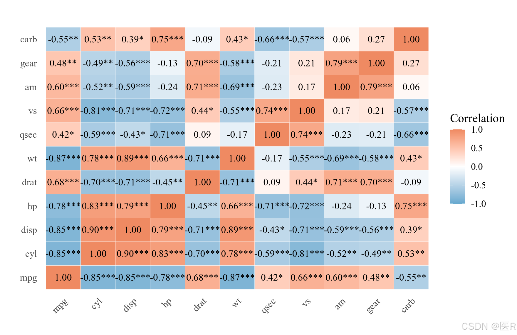
ggplot2绘制三角热图
R
library(Hmisc)
library(reshape2)
library(ggplot2)

# 准备数据
df <- mtcars
res <- rcorr(as.matrix(df))
r_mat <- res$r
p_mat <- res$P

# 转长格式
r_df <- melt(r_mat, na.rm = FALSE)
p_df <- melt(p_mat, na.rm = FALSE)

# 显著性标记
p_df$signif <- cut(p_df$value,
                   breaks = c(-Inf, 0.001, 0.01, 0.05, Inf),
                   labels = c("***", "**", "*", ""))

# 合并
plot_df <- merge(r_df, p_df, by = c("Var1", "Var2"))
plot_df$signif[plot_df$Var1 == plot_df$Var2] <- ""
plot_df$label <- paste0(sprintf("%.2f", plot_df$value.x), plot_df$signif)

# 只保留右上三角格子(包含对角线)
plot_df <- plot_df[as.numeric(plot_df$Var2) >= as.numeric(plot_df$Var1), ]

# 构造对角线上方的变量名标签
diagonal_labels <- subset(plot_df, Var1 == Var2)
diagonal_labels$label <- as.character(diagonal_labels$Var1)
diagonal_labels$y_pos <- as.numeric(diagonal_labels$Var1) - 0.3  # 微微往上移

# 绘图

ggplot() +
  geom_tile(data = plot_df, aes(x = Var2, y = Var1, fill = value.x), color = "white") +
  geom_text(data = plot_df, aes(x = Var2, y = Var1, label = label),
            family = "Times New Roman", size = 4) +
  geom_text(data = diagonal_labels, aes(x = Var2, y = y_pos+1, label = label),
            family = "Times New Roman",  size = 4) +
  scale_fill_gradient2(
    low = "#67a9cf", high = "#ef8a62", mid = "white",
    midpoint = 0, limit = c(-1, 1), name = "Correlation",
    labels = scales::number_format(accuracy = 0.1)
  ) +
  # coord_fixed() +  #  保持格子为正方形
  labs(title = "", x = "", y = "") +
  theme_minimal(base_size = 14) +
  expand_limits(y = max(as.numeric(plot_df$Var1)) + 1)+
  theme(
    axis.text.y = element_blank(),
    axis.ticks.y = element_blank(),
    axis.text.x = element_text(angle = 45, hjust = 1),
    panel.grid = element_blank(),
    text = element_text(family = "Times New Roman"),
    plot.title = element_text(hjust = 0.5)
  )
结果展示03:

corrplot绘制三角热图
R
# 示例数据
df <- mtcars
cor_matrix <- cor(df)

par(family = "Times New Roman")

corrplot(cor_matrix,
         method = "square",        # 方格图
         type = "upper",           # 只显示上三角
         diag = TRUE,              # 显示对角线
         addCoef.col = "black",    # 显示相关系数数字
         number.cex = 0.7,         # 数值大小
         tl.col = "black",         # 标签颜色
         tl.cex = 0.8,             # 标签字体大小
         tl.srt = 45,              # x轴标签角度(支持 45°/60° 等)
         col = colorRampPalette(c("#67a9cf", "white", "#ef8a62"))(200),
         mar = c(0,0,2,0)          # 边距微调
)
结果展示04:
