使用PyTorch 的神经网络模型对三维点云数据进行分类

1. 概述

本代码旨在构建一个基于 PyTorch 的神经网络模型，用于对生成的三维点云数据进行分类。通过生成数据集、数据预处理、模型训练、评估以及可视化等一系列操作，展示了一个完整的深度学习分类任务流程。最终通过绘制决策曲面和损失曲线，直观地呈现模型的性能和训练过程。

2. 依赖库导入

python

import numpy as np
import matplotlib.pyplot as plt
from mpl_toolkits.mplot3d import Axes3D
import torch
import torch.nn as nn
import torch.optim as optim
from sklearn.datasets import make_classification
from sklearn.model_selection import train_test_split
from sklearn.preprocessing import StandardScaler
from sklearn.metrics import accuracy_score
from matplotlib.colors import ListedColormap
from torchviz import make_dot
from matplotlib import cm

• numpy：作为 Python 科学计算的基础库，提供了高效的数组操作和数值计算功能，用于处理数据的各种数学运算。
• matplotlib.pyplot：是 Python 中常用的绘图库，用于创建各种静态、动态和交互式可视化图表，在本代码中用于绘制损失曲线和决策曲面。
• Axes3D：matplotlib的一个子模块，专门用于创建三维图形，以可视化三维点云数据的决策曲面。
• torch：PyTorch 深度学习框架的核心库，提供了张量操作、自动求导等功能，是构建和训练神经网络的基础。
• torch.nn：包含了 PyTorch 中用于构建神经网络的各种模块和层，如全连接层、激活函数层、归一化层等，方便用户构建复杂的神经网络模型。
• torch.optim：提供了多种优化算法，如随机梯度下降（SGD）、Adam 等，用于在训练过程中更新神经网络的参数，以最小化损失函数。
• make_classification：sklearn库中的函数，用于生成人工合成的分类数据集，可指定样本数量、特征数量、类别数量等参数。
• train_test_split：用于将数据集分割为训练集和测试集，方便对模型进行训练和评估。
• StandardScaler：数据预处理工具，用于对数据进行标准化处理，使每个特征的均值为 0，标准差为 1，有助于提高模型的训练效果和收敛速度。
• accuracy_score：用于计算分类模型的准确率，衡量模型预测结果与真实标签的匹配程度。
• ListedColormap：matplotlib中的类，用于创建自定义颜色映射，以便在绘制决策曲面和数据点时使用不同的颜色表示不同的类别。
• make_dot：torchviz库中的函数，用于生成 PyTorch 模型的计算图，帮助理解模型的结构和计算流程。
• cm：matplotlib的颜色映射模块，提供了多种预定义的颜色映射方案，可用于可视化。

3. 生成三维散点数据

python

np.random.seed(42)
X, y = make_classification(n_samples=500, n_features=3, n_redundant=0,
                          n_informative=3, n_classes=3, n_clusters_per_class=1,
                          class_sep=1.8, random_state=42)

• np.random.seed(42)：设置随机数种子为 42，确保每次运行代码时生成的随机数序列相同，从而使生成的数据集具有可重复性。
• make_classification函数的参数说明：
  • n_samples：指定生成的样本数量为 500 个。
  • n_features：表示每个样本的特征数量为 3 个，即生成的是三维点云数据。
  • n_redundant：设置为 0，表示生成的数据中没有冗余特征。
  • n_informative：设为 3，意味着有 3 个对分类有贡献的信息性特征。
  • n_classes：指定数据的类别数量为 3 类。
  • n_clusters_per_class：每个类别包含 1 个簇。
  • class_sep：设置为 1.8，控制不同类别之间的分离程度，值越大，类别之间的区分越明显。
  • random_state：同样设置为 42，进一步保证生成数据集的随机性是可复现的。
• 执行后，X是一个形状为(500, 3)的numpy数组，存储了生成的 500 个样本的三维特征数据；y是一个形状为(500,)的numpy数组，存储了每个样本对应的类别标签（0、1 或 2）。

4. 数据预处理和转换为张量

python

scaler = StandardScaler()
X = scaler.fit_transform(X)
X_tensor = torch.FloatTensor(X)
y_tensor = torch.LongTensor(y)

• scaler = StandardScaler()：创建一个StandardScaler对象，用于对数据进行标准化处理。
• X = scaler.fit_transform(X)：fit方法计算数据的均值和标准差等统计信息，transform方法根据这些统计信息对原始数据X进行标准化，使得每个特征的均值为 0，标准差为 1。经过处理后，X仍然是一个形状为(500, 3)的numpy数组。
• X_tensor = torch.FloatTensor(X)：将标准化后的numpy数组X转换为 PyTorch 的FloatTensor类型，以便输入到神经网络中进行计算。此时X_tensor的形状为(500, 3)。
• y_tensor = torch.LongTensor(y)：将存储类别标签的numpy数组y转换为 PyTorch 的LongTensor类型，因为在分类任务中，通常使用整数类型表示类别标签。y_tensor的形状为(500,)。

5. 分割数据集

python

X_train, X_test, y_train, y_test = train_test_split(X_tensor, y_tensor, test_size=0.3, random_state=42)

• train_test_split函数用于将数据集分割为训练集和测试集。
• 参数X_tensor和y_tensor分别是之前转换好的输入特征张量和类别标签张量。
• test_size=0.3表示将数据集的 30% 作为测试集，其余 70% 作为训练集。
• random_state=42再次设置随机种子，确保每次分割数据集的结果都是相同的，保证实验的可重复性。
• 分割后，X_train和y_train用于训练神经网络模型，X_test和y_test用于评估模型的性能。

6. 定义神经网络模型

python

class PointCloudClassifier(nn.Module):
    def __init__(self):
        super(PointCloudClassifier, self).__init__()
        self.fc1 = nn.Linear(3, 64)
        self.bn1 = nn.BatchNorm1d(64)
        self.fc2 = nn.Linear(64, 128)
        self.bn2 = nn.BatchNorm1d(128)
        self.fc3 = nn.Linear(128, 64)
        self.bn3 = nn.BatchNorm1d(64)
        self.fc4 = nn.Linear(64, 3)
        self.dropout = nn.Dropout(0.3)
        self.relu = nn.ReLU()
    
    def forward(self, x):
        x = self.relu(self.bn1(self.fc1(x)))
        x = self.dropout(x)
        x = self.relu(self.bn2(self.fc2(x)))
        x = self.dropout(x)
        x = self.relu(self.bn3(self.fc3(x)))
        x = self.dropout(x)
        x = self.fc4(x)
        return x

• 定义了一个名为PointCloudClassifier的类，继承自nn.Module，这是 PyTorch 中所有神经网络模型的基类。
• __init__方法是类的构造函数，用于初始化神经网络的层和参数：
  • self.fc1 = nn.Linear(3, 64)：创建第一个全连接层，输入维度为 3（对应三维点云数据的特征数量），输出维度为 64，即该层将每个样本的 3 维特征映射到 64 维空间。
  • self.bn1 = nn.BatchNorm1d(64)：为第一个全连接层的输出添加批量归一化层，用于加速训练过程并提高模型的稳定性，归一化的维度为 64。
  • self.fc2 = nn.Linear(64, 128)：第二个全连接层，将 64 维的输入映射到 128 维空间。
  • self.bn2 = nn.BatchNorm1d(128)：对第二个全连接层的输出进行批量归一化，归一化维度为 128。
  • self.fc3 = nn.Linear(128, 64)：第三个全连接层，将 128 维的输入映射回 64 维空间。
  • self.bn3 = nn.BatchNorm1d(64)：对第三个全连接层的输出进行批量归一化，归一化维度为 64。
  • self.fc4 = nn.Linear(64, 3)：最后一个全连接层，将 64 维的输入映射到 3 维空间，对应 3 个类别，输出的结果将用于计算每个样本属于各个类别的概率。
  • self.dropout = nn.Dropout(0.3)：创建一个 Dropout 层，以 0.3 的概率随机丢弃神经元，防止模型过拟合。
  • self.relu = nn.ReLU()：创建 ReLU 激活函数层，用于引入非线性，使模型能够学习到更复杂的模式。
• forward方法定义了数据在神经网络中的前向传播路径：
  • 输入数据x首先经过第一个全连接层fc1，然后通过批量归一化层bn1，再经过 ReLU 激活函数，得到激活后的输出。
  • 对激活后的输出应用 Dropout 层，随机丢弃部分神经元。
  • 按照上述类似的方式，依次经过后续的全连接层、批量归一化层、ReLU 激活函数和 Dropout 层，直到最后一个全连接层fc4输出最终结果。

7. 初始化模型

python

model = PointCloudClassifier()
criterion = nn.CrossEntropyLoss()
optimizer = optim.Adam(model.parameters(), lr=0.001)

• model = PointCloudClassifier()：创建PointCloudClassifier类的实例，即初始化我们定义的神经网络模型。
• criterion = nn.CrossEntropyLoss()：选择交叉熵损失函数作为模型的损失度量。在多分类问题中，交叉熵损失函数常用于衡量预测概率分布与真实标签之间的差异。
• optimizer = optim.Adam(model.parameters(), lr=0.001)：使用 Adam 优化器来更新模型的参数。model.parameters()获取模型中所有需要更新的参数（权重和偏置），lr=0.001设置学习率为 0.001，控制每次参数更新的步长。

8. 训练模型

python

num_epochs = 300
train_losses = []
test_losses = []

for epoch in range(num_epochs):
    model.train()
    optimizer.zero_grad()
    outputs = model(X_train)
    loss = criterion(outputs, y_train)
    loss.backward()
    optimizer.step()
    train_losses.append(loss.item())
    
    model.eval()
    with torch.no_grad():
        test_outputs = model(X_test)
        test_loss = criterion(test_outputs, y_test)
        test_losses.append(test_loss.item())
    
    if (epoch+1) % 50 == 0:
        print(f'Epoch [{epoch+1}/{num_epochs}], Loss: {loss.item():.4f}, Test Loss: {test_loss.item():.4f}')

• num_epochs = 300：设置训练的轮数为 300 次，即让模型对整个训练集进行 300 次迭代训练。
• train_losses = []和test_losses = []：分别创建两个空列表，用于存储每一轮训练的训练损失和测试损失。
• 在每个训练轮次中：
  • model.train()：将模型设置为训练模式，此时 Dropout 层和批量归一化层会按照训练时的方式进行操作（如 Dropout 会随机丢弃神经元，批量归一化会根据当前批次的数据计算均值和方差）。
  • optimizer.zero_grad()：将优化器的梯度清零，因为在 PyTorch 中，梯度是累加的，每次迭代前需要将梯度设置为 0，否则会导致梯度计算错误。
  • outputs = model(X_train)：将训练集数据X_train输入到模型中，进行前向传播，得到模型的输出outputs，其形状为(训练样本数量, 类别数量)，即每个样本属于各个类别的概率。
  • loss = criterion(outputs, y_train)：根据模型的输出outputs和训练集的真实标签y_train，使用交叉熵损失函数计算损失值。
  • loss.backward()：进行反向传播，计算损失函数对模型参数的梯度。
  • optimizer.step()：根据计算得到的梯度，使用 Adam 优化器更新模型的参数，以最小化损失函数。
  • train_losses.append(loss.item())：将当前轮次的训练损失值添加到train_losses列表中。
  • model.eval()：将模型设置为评估模式，此时 Dropout 层不再随机丢弃神经元，批量归一化层使用训练时计算得到的均值和方差（而不是当前批次的数据），以确保评估结果的稳定性。
  • with torch.no_grad()：在这个代码块内，不会计算梯度，从而节省内存并加快计算速度。用于对测试集进行前向传播，得到测试集的输出test_outputs。
  • test_loss = criterion(test_outputs, y_test)：根据测试集的输出test_outputs和测试集的真实标签y_test，计算测试损失值。
  • test_losses.append(test_loss.item())：将当前轮次的测试损失值添加到test_losses列表中。
  • if (epoch+1) % 50 == 0:：每训练 50 轮，打印当前轮次的训练损失和测试损失，以便观察模型的训练进展和性能变化。

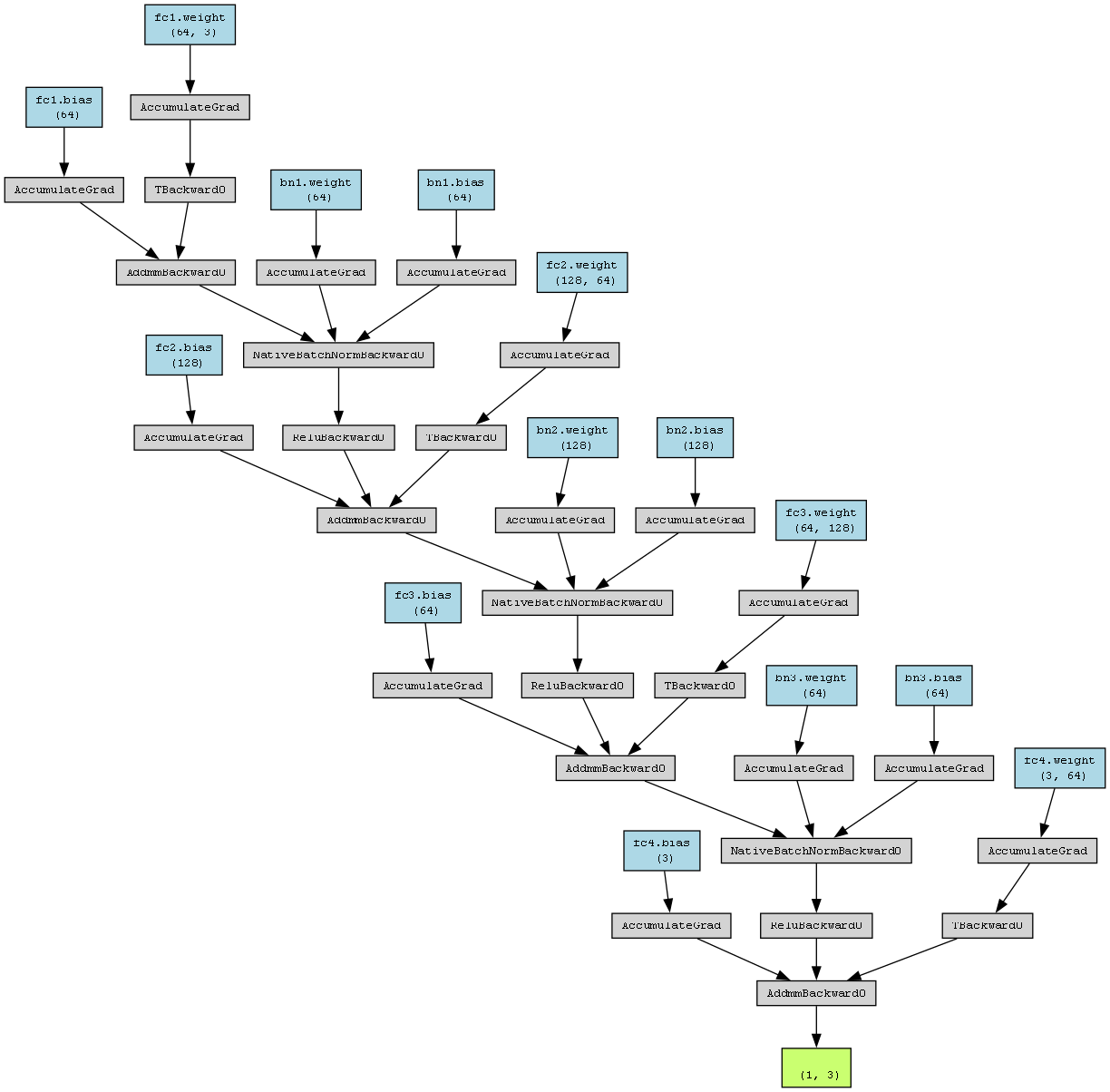
9. 生成计算图

python

dummy_input = torch.randn(1, 3)
make_dot(model(dummy_input), params=dict(model.named_parameters())).render("point_cloud_model", format="png")

• dummy_input = torch.randn(1, 3)：创建一个形状为(1, 3)的随机张量，作为模型的虚拟输入。这里的形状(1, 3)与模型输入的维度要求一致，即一个样本的三维特征数据。
• make_dot(model(dummy_input), params=dict(model.named_parameters()))：使用make_dot函数生成模型的计算图。model(dummy_input)将虚拟输入传入模型，得到模型的输出，params=dict(model.named_parameters())传入模型的参数，以便在计算图中显示参数信息。
• .render("point_cloud_model", format="png")：将生成的计算图保存为名为point_cloud_model的 PNG 格式图片，方便可视化模型的结构和计算流程。

10. 评估模型

python

model.eval()
with torch.no_grad():
    train_pred = model(X_train).argmax(dim=1).numpy()
    test_pred = model(X_test).argmax(dim=1).numpy()
    
print(f"训练集准确率: {accuracy_score(y_train.numpy(), train_pred):.4f}")
print(f"测试集准确率: {accuracy_score(y_test.numpy(), test_pred):.4f}")

• model.eval()：将模型设置为评估模式，确保在评估过程中模型的行为是稳定的（如 Dropout 层不工作，批量归一化层使用固定的统计信息）。
• with torch.no_grad()：在这个代码块内，不计算梯度，提高计算效率。
  • train_pred = model(X_train).argmax(dim=1).numpy()：将训练集数据X_train输入到模型中，得到模型的输出，然后使用argmax(dim=1)函数获取每个样本预测概率最大的类别索引，最后将结果转换为numpy数组，得到训练集的预测标签train_pred。
  • test_pred = model(X_test).argmax(dim=1).numpy()：对测试集数据X_test进行同样的操作，得到测试集的预测标签test_pred。
• accuracy_score(y_train.numpy(), train_pred)和accuracy_score(y_test.numpy(), test_pred)：分别计算训练集和测试集的准确率，即将预测标签与真实标签进行比较，计算预测正确的样本占总样本的比例。最后打印出训练集和测试集的准确率，以评估模型的性能。

11. 创建决策曲面可视化

python

def plot_decision_surface(model, X, y, feature1=0, feature2=1, fixed_value=0, title=""):
    fig = plt.figure(figsize=(10, 8))

计算图

完整代码

import numpy as np
import matplotlib.pyplot as plt
from mpl_toolkits.mplot3d import Axes3D
import torch
import torch.nn as nn
import torch.optim as optim
from sklearn.datasets import make_classification
from sklearn.model_selection import train_test_split
from sklearn.preprocessing import StandardScaler
from sklearn.metrics import accuracy_score
from matplotlib.colors import ListedColormap
from torchviz import make_dot
from matplotlib import cm

# 1. 生成三维散点数据
np.random.seed(42)
X, y = make_classification(n_samples=500, n_features=3, n_redundant=0,
                          n_informative=3, n_classes=3, n_clusters_per_class=1,
                          class_sep=1.8, random_state=42)

# 2. 数据预处理和转换为张量
scaler = StandardScaler()
X = scaler.fit_transform(X)
X_tensor = torch.FloatTensor(X)
y_tensor = torch.LongTensor(y)

# 3. 分割数据集
X_train, X_test, y_train, y_test = train_test_split(X_tensor, y_tensor, test_size=0.3, random_state=42)

# 4. 定义神经网络模型
class PointCloudClassifier(nn.Module):
    def __init__(self):
        super(PointCloudClassifier, self).__init__()
        self.fc1 = nn.Linear(3, 64)
        self.bn1 = nn.BatchNorm1d(64)
        self.fc2 = nn.Linear(64, 128)
        self.bn2 = nn.BatchNorm1d(128)
        self.fc3 = nn.Linear(128, 64)
        self.bn3 = nn.BatchNorm1d(64)
        self.fc4 = nn.Linear(64, 3)
        self.dropout = nn.Dropout(0.3)
        self.relu = nn.ReLU()
    
    def forward(self, x):
        x = self.relu(self.bn1(self.fc1(x)))
        x = self.dropout(x)
        x = self.relu(self.bn2(self.fc2(x)))
        x = self.dropout(x)
        x = self.relu(self.bn3(self.fc3(x)))
        x = self.dropout(x)
        x = self.fc4(x)
        return x

# 5. 初始化模型
model = PointCloudClassifier()
criterion = nn.CrossEntropyLoss()
optimizer = optim.Adam(model.parameters(), lr=0.001)

# 6. 训练模型
num_epochs = 300
train_losses = []
test_losses = []

for epoch in range(num_epochs):
    model.train()
    optimizer.zero_grad()
    outputs = model(X_train)
    loss = criterion(outputs, y_train)
    loss.backward()
    optimizer.step()
    train_losses.append(loss.item())
    
    model.eval()
    with torch.no_grad():
        test_outputs = model(X_test)
        test_loss = criterion(test_outputs, y_test)
        test_losses.append(test_loss.item())
    
    if (epoch+1) % 50 == 0:
        print(f'Epoch [{epoch+1}/{num_epochs}], Loss: {loss.item():.4f}, Test Loss: {test_loss.item():.4f}')

# 7. 生成计算图
dummy_input = torch.randn(1, 3)
make_dot(model(dummy_input), params=dict(model.named_parameters())).render("point_cloud_model", format="png")

# 8. 评估模型
model.eval()
with torch.no_grad():
    train_pred = model(X_train).argmax(dim=1).numpy()
    test_pred = model(X_test).argmax(dim=1).numpy()
    
print(f"训练集准确率: {accuracy_score(y_train.numpy(), train_pred):.4f}")
print(f"测试集准确率: {accuracy_score(y_test.numpy(), test_pred):.4f}")

# 9. 创建决策曲面可视化
def plot_decision_surface(model, X, y, feature1=0, feature2=1, fixed_value=0, title=""):
    fig = plt.figure(figsize=(10, 8))
    ax = fig.add_subplot(111, projection='3d')
    
    # 创建网格
    x_min, x_max = X[:, feature1].min() - 1, X[:, feature1].max() + 1
    y_min, y_max = X[:, feature2].min() - 1, X[:, feature2].max() + 1
    xx, yy = np.meshgrid(np.linspace(x_min, x_max, 50),
                         np.linspace(y_min, y_max, 50))
    
    # 预测每个网格点的类别
    with torch.no_grad():
        if feature1 == 0 and feature2 == 1:
            grid_input = np.column_stack((xx.ravel(), yy.ravel(), np.full_like(xx.ravel(), fixed_value)))
        elif feature1 == 0 and feature2 == 2:
            grid_input = np.column_stack((xx.ravel(), np.full_like(xx.ravel(), fixed_value), yy.ravel()))
        else:
            grid_input = np.column_stack((np.full_like(xx.ravel(), fixed_value), xx.ravel(), yy.ravel()))
            
        grid_tensor = torch.FloatTensor(grid_input)
        Z = model(grid_tensor).argmax(dim=1).numpy()
        Z = Z.reshape(xx.shape)
    
    # 绘制曲面
    surf = ax.plot_surface(xx, yy, Z, cmap=ListedColormap(['#FF0000', '#00FF00', '#0000FF']), 
                          alpha=0.3, antialiased=True)
    
    # 绘制原始数据点
    scatter = ax.scatter(X[:, feature1], X[:, feature2], X[:, 3 - feature1 - feature2], 
                        c=y, cmap=ListedColormap(['#FF0000', '#00FF00', '#0000FF']),
                        s=40, edgecolors='k')
    
    ax.set_title(title)
    ax.set_xlabel(f'Feature {feature1+1}')
    ax.set_ylabel(f'Feature {feature2+1}')
    ax.set_zlabel(f'Feature {3 - feature1 - feature2+1}')
    plt.colorbar(surf, ax=ax, shrink=0.5, aspect=5)
    plt.show()

# 10. 绘制三个不同视角的决策曲面
plot_decision_surface(model, X, y, feature1=0, feature2=1, fixed_value=0, title="Decision Surface (Fixed Feature 3=0)")
plot_decision_surface(model, X, y, feature1=0, feature2=2, fixed_value=0, title="Decision Surface (Fixed Feature 2=0)")
plot_decision_surface(model, X, y, feature1=1, feature2=2, fixed_value=0, title="Decision Surface (Fixed Feature 1=0)")

# 11. 可视化训练过程
plt.figure(figsize=(10, 5))
plt.plot(train_losses, label='Training Loss')
plt.plot(test_losses, label='Test Loss')
plt.title('Training and Test Loss Over Epochs')
plt.xlabel('Epoch')
plt.ylabel('Loss')
plt.legend()
plt.show()