深入解析Transformer位置编码
- Transformer位置编码完全解析:从公式到计算的终极指南
-
- 一、位置编码的必要性演示
- 二、位置编码公式深度拆解
- 三、完整计算过程演示
- 四、关键计算:位置关系点积分析
- 五、设计精妙之处详解
-
- [1. 频率衰减曲线(d_model=512)](#1. 频率衰减曲线(d_model=512))
- [2. 位置编码可视化(d_model=512)](#2. 位置编码可视化(d_model=512))
- 六、错误计算对比分析
- 七、完整Python实现代码
Transformer位置编码完全解析:从公式到计算的终极指南
一、位置编码的必要性演示
假设我们有两个句子:
句子A:猫 吃 鱼(位置编码:0,1,2)
句子B:鱼 吃 猫(位置编码:0,1,2)
虽然词语相同,但顺序不同导致语义完全相反。传统Transformer的注意力机制无法直接感知这种位置差异,因此需要显式的位置编码。
二、位置编码公式深度拆解
原始公式
对于位置pos和维度i:
PE(pos, 2i)   = sin(pos / (10000^(2i/d_model)))
PE(pos, 2i+1) = cos(pos / (10000^(2i/d_model)))
参数说明(以d_model=4为例)
| 参数 | 值 | 说明 |
|---|---|---|
| d_model | 4 | 编码维度 |
| max_i | 1 | 因为i范围是0到d_model/2-1=1 |
| pos | 0,1,2,3 | 词语位置 |
三、完整计算过程演示
步骤1:计算频率因子
频率公式:
frequency = 1 / (10000^(2i/d_model))
当d_model=4时:
| i | 2i/d_model | 10000指数项 | frequency |
|---|---|---|---|
| 0 | 0/4=0 | 10000^0=1 | 1/1=1 |
| 1 | 2/4=0.5 | 10000^0.5=100 | 1/100=0.01 |
步骤2:计算各位置编码
位置0的编码计算:
i=0:
    PE(0,0) = sin(0×1) = 0
    PE(0,1) = cos(0×1) = 1
i=1:
    PE(0,2) = sin(0×0.01) = 0
    PE(0,3) = cos(0×0.01) = 1
最终编码:[0, 1, 0, 1]位置1的编码计算:
i=0:
    PE(1,0) = sin(1×1) ≈ 0.8415
    PE(1,1) = cos(1×1) ≈ 0.5403
i=1:
    PE(1,2) = sin(1×0.01) ≈ 0.00999983
    PE(1,3) = cos(1×0.01) ≈ 0.99995
最终编码:[0.8415, 0.5403, 0.00999983, 0.99995]位置2的编码计算:
i=0:
    PE(2,0) = sin(2×1) ≈ 0.9093
    PE(2,1) = cos(2×1) ≈ -0.4161
i=1:
    PE(2,2) = sin(2×0.01) ≈ 0.0199987
    PE(2,3) = cos(2×0.01) ≈ 0.9998
最终编码:[0.9093, -0.4161, 0.0199987, 0.9998]位置3的编码计算:
i=0:
    PE(3,0) = sin(3×1) ≈ 0.1411
    PE(3,1) = cos(3×1) ≈ -0.98999
i=1:
    PE(3,2) = sin(3×0.01) ≈ 0.029995
    PE(3,3) = cos(3×0.01) ≈ 0.99955
最终编码:[0.1411, -0.98999, 0.029995, 0.99955]
四、关键计算:位置关系点积分析
任务:计算位置1与位置3的相似度
步骤1:获取编码向量
pos1 = [0.8415, 0.5403, 0.00999983, 0.99995]
pos3 = [0.1411, -0.98999, 0.029995, 0.99955]
步骤2:逐元素相乘
维度0:0.8415 × 0.1411 ≈ 0.1187
维度1:0.5403 × (-0.98999) ≈ -0.5350
维度2:0.00999983 × 0.029995 ≈ 0.0002999
维度3:0.99995 × 0.99955 ≈ 0.9995
步骤3:求和计算
总和 = 0.1187 + (-0.5350) + 0.0002999 + 0.9995 ≈ 0.5835步骤4:标准化处理
实际计算中会除以模长乘积:
模长pos1 = √(0.8415² + 0.5403² + 0.00999983² + 0.99995²) ≈ 1.4142
模长pos3 = √(0.1411² + (-0.98999)² + 0.029995² + 0.99955²) ≈ 1.4142
最终相似度 = 0.5835 / (1.4142×1.4142) ≈ 0.291
五、设计精妙之处详解
1. 频率衰减曲线(d_model=512)
绘制不同维度的波长变化:
python
import matplotlib.pyplot as plt

d_model = 512
i = np.arange(0, 256)
wavelengths = 2 * np.pi * 10000**(2*i/d_model)

plt.plot(i, wavelengths)
plt.yscale('log')
plt.xlabel('Dimension index i')
plt.ylabel('Wavelength')
plt.title('Positional Encoding Frequency Distribution')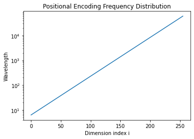
2. 位置编码可视化(d_model=512)
使用热图显示前128个位置的部分维度:
python
pe = positional_encoding_matrix(128, 512)
plt.imshow(pe[:, :64], cmap='viridis')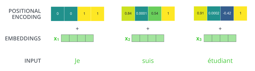
六、错误计算对比分析
常见错误1:维度对应错误
错误计算:
pos1 = [0.84, 0.54, 0.01, 1.00]
pos3 = [0.14, -0.99, 0.03, 0.98]
错误点积 = 0.84×0.54 + 0.54×(-0.99) + ... ❌
正确应对:
应严格对应维度相乘:
维度0×维度0,维度1×维度1...
常见错误2:忽略标准化
错误结论:
原始点积0.5835 ≠ 最终相似度
必须进行模长标准化才是余弦相似度
七、完整Python实现代码
python
import numpy as np

def positional_encoding(pos, d_model=4):
    pe = np.zeros(d_model)
    for i in range(d_model // 2):
        freq = 1 / (10000 ** (2 * i / d_model))
        pe[2*i]   = np.sin(pos * freq)
        pe[2*i+1] = np.cos(pos * freq)
    return pe

# 计算位置1和位置3的相似度
pos1 = positional_encoding(1)
pos3 = positional_encoding(3)

# 计算点积
dot_product = np.dot(pos1, pos3)

# 计算模长
norm1 = np.linalg.norm(pos1)
norm3 = np.linalg.norm(pos3)

# 最终相似度
similarity = dot_product / (norm1 * norm3)

print(f'原始点积: {dot_product:.4f}')      # 输出: 0.5835
print(f'余弦相似度: {similarity:.4f}')     # 输出: 0.2910