机器学习课堂7用scikit-learn库训练SVM模型

1.用scikit-learn库训练SVM模型

代码

#  2-11用scikit-learn库训练SVM模型
import pandas as pd
import numpy as np
import matplotlib.pyplot as plt
from sklearn import svm  # 导入sklearn

# 参数设置
m_train = 250  # 训练样本数量
svm_C = 100  # SVM的C值
svm_kernel = 'linear'  # SVM的核函数
# 读入酒驾检测数据集
df = pd.read_csv('alcohol_dataset.csv')
data = np.array(df)
m_all = np.shape(data)[0]  # 样本总数
d = np.shape(data)[1] - 1  # 输入特征的维数
m_test = m_all - m_train  # 测试数据集样本数量
# 把0标注替换为-1
data[:, d] = np.where(data[:, d] == 0, -1, data[:, d])
# 构造随机种子为指定值的随机数生成器，并对数据集中样本随机排序
rng = np.random.default_rng(1)
rng.shuffle(data)
mean = np.mean(data[0:m_train, 0:d], axis=0)  # 计算训练样本输入特征的均值
std = np.std(data[0:m_train, 0:d], axis=0, ddof=1)  # 计算训练样本输入特诊的标准差
data[:, 0:d] = (data[:, 0:d] - mean) / std  # 标准化所有样本的输入特征
# 划分数据集
X_train = data[0:m_train, 0:d]  # 训练集输入特征
X_test = data[m_train:, 0:d]  # 测试集输入特征
Y_train = data[0:m_train, d]  # 训练集目标值
Y_test = data[m_train:, d]  # 测试集目标值
#  SVM训练与预测
clf = svm.SVC(kernel=svm_kernel, C=svm_C)
clf.fit(X_train, Y_train)  # 训练
Y_train_hat = clf.predict(X_train)  # 训练数据集上的预测
Y_test_hat = clf.predict(X_test)  # 测试数据集上的预测
# 打印分类错误的数量
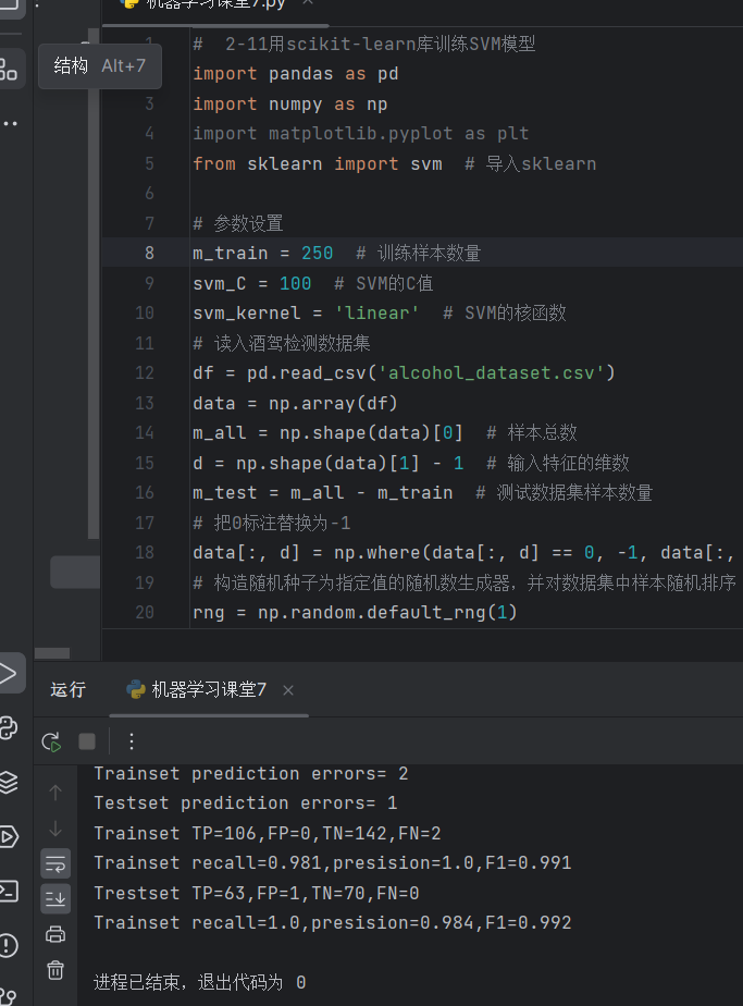
print('Trainset prediction errors=', np.sum(Y_train != Y_train_hat))
print('Testset prediction errors=', np.sum(Y_test != Y_test_hat))
# 训练数据集上的混淆矩阵
tp = np.sum(np.logical_and(Y_train == 1, Y_train_hat == 1))  # TP
fp = np.sum(np.logical_and(Y_train == -1, Y_train_hat == 1))  # FP
tn = np.sum(np.logical_and(Y_train == -1, Y_train_hat == -1))  # TN
fn = np.sum(np.logical_and(Y_train == 1, Y_train_hat == -1))  # FN
print(f'Trainset TP={tp},FP={fp},TN={tn},FN={fn}')
# 训练数据集上的召回率、精度、F1值
recall = tp / (tp + fn)
precision = tp / (tp + fp)
f1 = 2 * recall * precision / (recall + precision)
print(f'Trainset recall={recall:.3},presision={precision:.3},F1={f1:.3}')
# 测试数据集上的混淆矩阵
tp_test = np.sum(np.logical_and(Y_test == 1, Y_test_hat == 1))
fp_test = np.sum(np.logical_and(Y_test == -1, Y_test_hat == 1))
tn_test = np.sum(np.logical_and(Y_test == -1, Y_test_hat == -1))
fn_test = np.sum(np.logical_and(Y_test == 1, Y_test_hat == -1))
print(f'Trestset TP={tp_test},FP={fp_test},TN={tn_test},FN={fn_test}')
# 测试数据集上的召回率、精度、F1值
recall_test = tp_test / (tp_test + fn_test)
precision_test = tp_test / (tp_test + fp_test)
f1_test = 2 * recall_test * precision_test / (recall_test + precision_test)
print(f'Trainset recall={recall_test:.3},presision={precision_test:.3},F1={f1_test:.3}')

结果

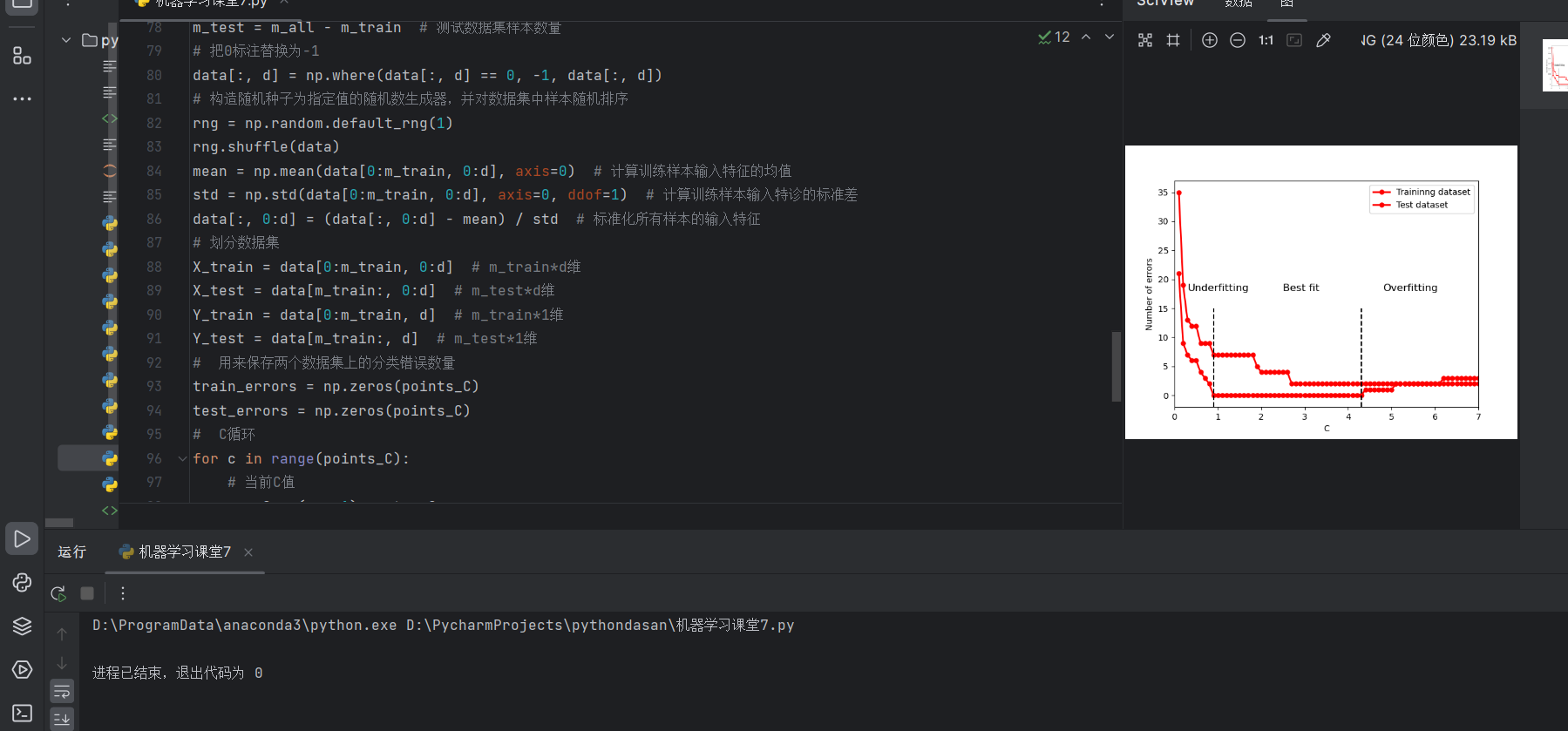
2.SVM模型的分类错误数量随C值变化的曲线

#  2-12画出SVM模型都分类错误数量随C值变化的曲线
import pandas as pd
import numpy as np
import matplotlib.pyplot as plt
from sklearn import svm  # 导入sklearn

# 参数设置
m_train = 250  # 训练样本数量
svm_kernel = 'poly'  # SVM的核函数
points_C = 70  # SVM的C值取值数量
step_C = 0.1  # C值的步长
# 读入酒驾检测数据集
df = pd.read_csv('alcohol_dataset.csv')
data = np.array(df)
m_all = np.shape(data)[0]  # 样本总数
d = np.shape(data)[1] - 1  # 输入特征的维数
m_test = m_all - m_train  # 测试数据集样本数量
# 把0标注替换为-1
data[:, d] = np.where(data[:, d] == 0, -1, data[:, d])
# 构造随机种子为指定值的随机数生成器，并对数据集中样本随机排序
rng = np.random.default_rng(1)
rng.shuffle(data)
mean = np.mean(data[0:m_train, 0:d], axis=0)  # 计算训练样本输入特征的均值
std = np.std(data[0:m_train, 0:d], axis=0, ddof=1)  # 计算训练样本输入特诊的标准差
data[:, 0:d] = (data[:, 0:d] - mean) / std  # 标准化所有样本的输入特征
# 划分数据集
X_train = data[0:m_train, 0:d]  # m_train*d维
X_test = data[m_train:, 0:d]  # m_test*d维
Y_train = data[0:m_train, d]  # m_train*1维
Y_test = data[m_train:, d]  # m_test*1维
#  用来保存两个数据集上的分类错误数量
train_errors = np.zeros(points_C)
test_errors = np.zeros(points_C)
#  C循环
for c in range(points_C):
    # 当前C值
    svm_C = (c + 1) * step_C
    # SVM训练与预测
    clf = svm.SVC(kernel=svm_kernel, C=svm_C)
    clf.fit(X_train, Y_train)  # 训练
    Y_train_hat = clf.predict(X_train)  # 训练数据集上的预测
    Y_test_hat = clf.predict(X_test)  # 测试数据集上的预测
    # 统计并保存两个数据集上的分类错误的数量
    train_errors[c] = np.sum(Y_train != Y_train_hat)
    test_errors[c] = np.sum(Y_test != Y_test_hat)
# 画出两条分类错误线
plt.plot(np.arange(1, points_C + 1) * step_C, train_errors, 'r-o', linewidth=2, markersize=5)
plt.plot(np.arange(1, points_C + 1) * step_C, test_errors, 'r-o', linewidth=2, markersize=5)
plt.ylabel('Number of errors')
plt.xlabel('C')
plt.legend(['Traininng dataset', 'Test dataset'])
plt.annotate('Underfitting', (0.3, 18), fontsize=12)
plt.annotate('Best fit', (2.5, 18), fontsize=12)
plt.annotate('Overfitting', (4.8, 18), fontsize=12)
plt.plot((0.9, 0.9), (-2, 15), '--k')
plt.plot((4.3, 4.3), (-2, 15), '--k')
plt.axis([0, 7, -2, 37])
plt.show()

结果图