其实是强化学习入门第一部分~
从问题定义到 Q-Learning 算法的提出。
1 任务背景
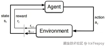
强化学习是一种学习如何从状态映射到动作 以最大化最终奖励的学习机制。智能体需要不断地在环境中进行实验,通过环境给予的反馈(奖励)来不断优化状态-行为的对应关系。
其中提及了四个要素,我们分别加以解释:
- 状态(State) :环境当前的情况,是智能体做决策的依据。
- 动作(Action) :智能体在某个状态下可以执行的操作。
- 奖励(Reward) :环境对智能体动作的即时反馈,决定行为的好坏。
- 策略(Policy) :智能体在特定状态下选择动作的规则,决定如何行动。
以 Breakout(打砖块) 为例,强化学习的任务可以概括为:让智能体通过不断试错,学习控制挡板击球,最大化清除砖块的得分,最终掌握高效连击和精准反弹的策略。
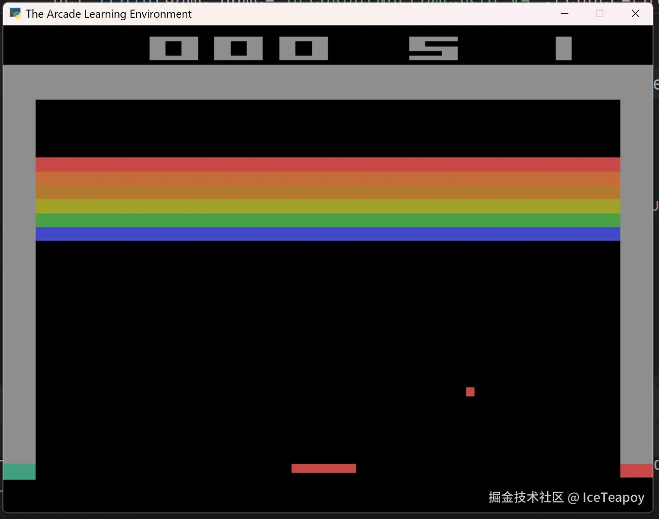
在打砖块游戏中,强化学习的四要素具体表现为:
| 要素 | Breakout示例 |
|---|---|
| 状态(State) | 历史游戏截图和操作序列 |
| 动作(Action) | 离散动作:左移、右移、不动 |
| 奖励(Reward) | 击碎砖块:+1,漏球:0,回合结束 |
| 策略(Policy) | 从当前状态到动作的映射函数 |
由此可以发现,与有监督学习和无监督学习相比,强化学习的任务具有以下特点:
- 从无标注的原始数据(视频、音频等)中学习。
- 奖励稀疏、嘈杂、延时。
- 数据间并不相互独立,而是具有时序性。
- 智能体的行为会影响后续的数据。
2 形式化问题定义
想要用算法解决问题,我们需要从具体问题中抽象出数学描述。
在强化学习框架中,智能体与环境的交互被建模为离散时间的马尔可夫决策过程(MDP),由元组 (S,A,R,P,γ) 构成。
2.1 变量定义
| 变量符号 | 定义 | 说明 |
|---|---|---|
| xt∈R | 当前时刻 t的原始像素观测(RGB图像) | 单帧游戏画面,未经过预处理 |
| at∈A | 离散动作空间(如{NOOP, FIRE, RIGHT, LEFT...}) | 对应游戏手柄的18种可能操作 |
| st∈S | 状态空间,历史帧画面和动作的序列: st=(x1,a1,x2,...,xt) | 过去游戏画面和执行操作依时序拼接形成的序列 |
| rt∈R | 游戏引擎返回的即时奖励 | 得分变化量(可能被裁剪到-1,1范围) |
| P(s′,r∣s,a) | 在状态 s 执行动作 a 后转移到状态 s′ 的概率并获得收益 r 的概率 | 状态转移概率函数,描述游戏环境 |
| γ | 折扣因子(论文中 γ=0.99) | 确保无限时域累计奖励收敛 |
2.2 强化学习的离散时间步过程
(1)状态观测
- 环境向智能体呈现当前状态 st∈S
- 状态是环境内部情况的完全或部分可观测表示
(2)动作选择
- 智能体根据内部策略生成动作 at∈A(st)
- A(st) 表示状态 st 下的可用动作集
(3)环境交互
- 动作 at 被传递至环境
- 环境根据内部动态特性产生:
- 新状态 st+1∼P(⋅∣st,at)
- 即时标量奖励 rt+1∈R
(4)信息传递
- 环境向智能体返回:
- 下一状态 st+1
- 奖励信号 rt+1
- 终止标志 dt+1∈{True,False}
(5)时间步推进
- 系统时钟从 t 递进到 t+1
- 若 dt+1=True,当前回合终止并重置环境
- 否则继续新一轮状态观测
3 Q-Learning 算法
智能体的决策是怎样产生的呢?
传统方法是提前制定固定规则(如棋类套路),或者将整个环境建模预处理最优解。像考试前背下所有题目答案,但遇到新题就会失败。
Q-Learning的突破在于:放弃对环境的完美认知,转而从实际经验中学习。这种设计让它能应对现实世界中的不确定性,但也需要更多试错数据(类似人类需要多次练习才能掌握技能)。
3.1 评价函数
我们在面临一个状态 s 的时候,怎样评价在该状态下执行操作 a 的好坏呢?要回答这个问题,我们需要建立一个能够同时考虑即时收益和长期影响的评价标准。由于强化学习任务中奖励的稀疏性和延时性,这个标准不仅要反映当前动作带来的直接回报,还要包含这个动作对未来可能状态的潜在影响。
比如《打砖块》游戏中,当球从右侧飞来时,智能体需要决定是将球拍向左移动还是向右移动。单次操作使球拍移动的距离可能很小,无法带来任何收益。此外,还应该考虑这个动作会导致球飞向哪个方向,进而影响后续能否连续击碎更多砖块。
为此,首先定义累计回报 Gt ------ 它表示从时刻 t 开始,未来所有奖励经过时间衰减后的总和:
Gt=rt+1+γrt+2+γ2rt+3+⋯=k=0∑∞γkrt+k+1=rt+1+γGt+1
其中 γ∈[0,1) 是折扣因子。这个设计既保证无穷级数收敛(当 γ<1时),又体现"近期奖励比远期更重要"的决策直觉。
首先考虑一个固定策略 π 的情况。假设我们有一个固定的行为规则,那么可以定义策略 π 下的动作价值函数:
Qπ(s,a)=EπGt∣st=s,at=a
这个函数表示在状态 s 下执行动作 a 后,继续按照策略 π 行动所能获得的期望累计回报。这里的期望是对策略 π 下所有可能轨迹的平均,就像记录一个固定打法的玩家千万次游戏的平均得分。
强化学习的目标是找到最优策略 π*,即在每个状态都能做出最佳决策的策略。这就引出了最优动作价值函数的概念:
Q∗(s,a)=πmaxQπ(s,a)
这个函数表示在所有可能的策略中,能够获得最大期望回报的那个策略对应的价值。理解这个区别很关键: Qπ 反映的是特定策略的表现,而 Q∗ 反映的是潜在的最佳表现。
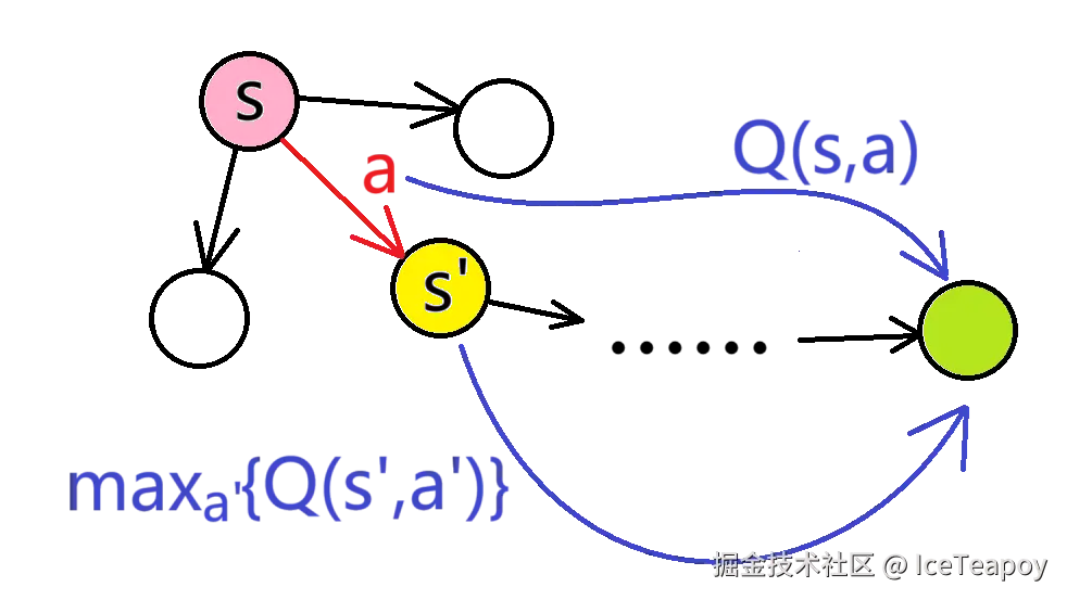
最优 Q 函数满足贝尔曼最优方程:
Q∗(s,a)=Er+γa′maxQ∗(s′,a′)
该方程将一个全局优化问题转化为局部递归关系。右边的 max 操作确保了我们在每个后续状态都会选择最优动作,从而保证整个策略的最优性。方程本质反映了动态规划的最优子结构特性:当前最优决策必须包含后续所有最优决策。
如果我们对贝尔曼方程进行递归预处理,提前求出 Q 表,就回归到了传统方法。面临着状态空间巨大、需要提前得知环境信息和无法应对环境改变等问题。
3.2 迭代规则
实践中,我们无法遍历所有可能的未来路径,于是通过采样单次转移 (s,a,r,s′) 构造迭代规则:
Q-Learning 的迭代规则是:
Q(s,a)←Q(s,a)+α(r+γa′maxQ(s′,a′)−Q(s,a))
即将 Q(s,a) 更新为 Q(s,a) 和 r+γmaxa′Q(s′,a′) 的加权平均数。
经过充分迭代后, Q 函数最终收敛到真实的最优价值评估。
这为后续 DQN 的发展奠定基础------用深度网络拟合 Q 函数。这种"从试错中建立价值认知"的范式,成为现代强化学习的核心方法论。