第R4周：LSTM-火灾温度预测

文章目录

一、前期准备工作
- 1.导入数据
- [2. 数据集可视化](#2. 数据集可视化)
二、构建数据集
- [1. 数据集预处理](#1. 数据集预处理)
- [2. 设置X, y](#2. 设置X, y)
- [3. 划分数据集](#3. 划分数据集)
三、模型训练
- [1. 构建模型](#1. 构建模型)
- [2. 定义训练函数](#2. 定义训练函数)
- [3. 定义测试函数](#3. 定义测试函数)
- [4. 正式训练模型](#4. 正式训练模型)
四、模型评估
- [1. Loss图片](#1. Loss图片)
- [2. 调用模型进行预测](#2. 调用模型进行预测)
- [3. R2值评估](#3. R2值评估)
总结：

🍨 本文为🔗365天深度学习训练营中的学习记录博客

🍖 原作者：K同学啊

一、前期准备工作

python 复制代码

import torch.nn.functional as F
import numpy  as np
import pandas as pd
import torch
from torch    import nn

1.导入数据

python 复制代码

data = pd.read_csv("woodpine2.csv")

data

| | Time | Tem1 | CO 1 | Soot 1 |
| 0 | 0.000 | 25.0 | 0.000000 | 0.000000 |
| 1 | 0.228 | 25.0 | 0.000000 | 0.000000 |
| 2 | 0.456 | 25.0 | 0.000000 | 0.000000 |
| 3 | 0.685 | 25.0 | 0.000000 | 0.000000 |
| 4 | 0.913 | 25.0 | 0.000000 | 0.000000 |
| ... | ... | ... | ... | ... |
| 5943 | 366.000 | 295.0 | 0.000077 | 0.000496 |
| 5944 | 366.000 | 294.0 | 0.000077 | 0.000494 |
| 5945 | 367.000 | 292.0 | 0.000077 | 0.000491 |
| 5946 | 367.000 | 291.0 | 0.000076 | 0.000489 |

5947	367.000	290.0	0.000076	0.000487

5948 rows × 4 columns

2. 数据集可视化

python 复制代码

import matplotlib.pyplot as plt
import seaborn as sns
 
plt.rcParams['savefig.dpi'] = 500 #图片像素
plt.rcParams['figure.dpi']  = 500 #分辨率
 
fig, ax =plt.subplots(1,3,constrained_layout=True, figsize=(14, 3))
 
sns.lineplot(data=data["Tem1"], ax=ax[0])
sns.lineplot(data=data["CO 1"], ax=ax[1])
sns.lineplot(data=data["Soot 1"], ax=ax[2])
plt.show()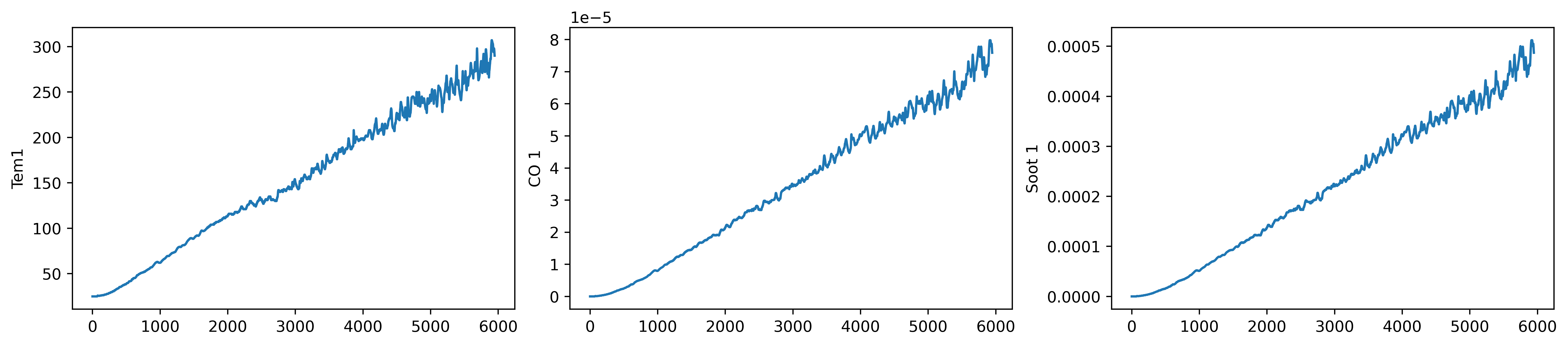

python 复制代码

dataFrame = data.iloc[:,1:]

dataFrame

| | Tem1 | CO 1 | Soot 1 |
| 0 | 25.0 | 0.000000 | 0.000000 |
| 1 | 25.0 | 0.000000 | 0.000000 |
| 2 | 25.0 | 0.000000 | 0.000000 |
| 3 | 25.0 | 0.000000 | 0.000000 |
| 4 | 25.0 | 0.000000 | 0.000000 |
| ... | ... | ... | ... |
| 5943 | 295.0 | 0.000077 | 0.000496 |
| 5944 | 294.0 | 0.000077 | 0.000494 |
| 5945 | 292.0 | 0.000077 | 0.000491 |
| 5946 | 291.0 | 0.000076 | 0.000489 |

5947	290.0	0.000076	0.000487

5948 rows × 3 columns

二、构建数据集

1. 数据集预处理

python 复制代码

from sklearn.preprocessing import MinMaxScaler

dataFrame = data.iloc[:,1:].copy()
sc  = MinMaxScaler(feature_range=(0, 1)) #将数据归一化，范围是0到1

for i in ['CO 1', 'Soot 1', 'Tem1']:
    dataFrame[i] = sc.fit_transform(dataFrame[i].values.reshape(-1, 1))

dataFrame.shape

复制代码

(5948, 3)

2. 设置X, y

python 复制代码

width_X = 8
width_y = 1

##取前8个时间段的Tem1、CO 1、Soot 1为X，第9个时间段的Tem1为y。
X = []
y = []

in_start = 0

for _, _ in data.iterrows():
    in_end  = in_start + width_X
    out_end = in_end   + width_y
    
    if out_end < len(dataFrame):
        X_ = np.array(dataFrame.iloc[in_start:in_end , ])
        y_ = np.array(dataFrame.iloc[in_end  :out_end, 0])

        X.append(X_)
        y.append(y_)
    
    in_start += 1

X = np.array(X)
y = np.array(y).reshape(-1,1,1)

X.shape, y.shape

复制代码

((5939, 8, 3), (5939, 1, 1))

检查数据集中是否有空值

python 复制代码

print(np.any(np.isnan(X)))
print(np.any(np.isnan(y)))

复制代码

False
False

3. 划分数据集

python 复制代码

X_train = torch.tensor(np.array(X[:5000]), dtype=torch.float32)
y_train = torch.tensor(np.array(y[:5000]), dtype=torch.float32)

X_test  = torch.tensor(np.array(X[5000:]), dtype=torch.float32)
y_test  = torch.tensor(np.array(y[5000:]), dtype=torch.float32)
X_train.shape, y_train.shape

复制代码

(torch.Size([5000, 8, 3]), torch.Size([5000, 1, 1]))

python 复制代码

from torch.utils.data import TensorDataset, DataLoader

train_dl = DataLoader(TensorDataset(X_train, y_train),
                      batch_size=64, 
                      shuffle=False)

test_dl  = DataLoader(TensorDataset(X_test, y_test),
                      batch_size=64, 
                      shuffle=False)

三、模型训练

1. 构建模型

python 复制代码

class model_lstm(nn.Module):
    def __init__(self):
        super(model_lstm, self).__init__()
        self.lstm0 = nn.LSTM(input_size=3 ,hidden_size=320, 
                             num_layers=1, batch_first=True)
        
        self.lstm1 = nn.LSTM(input_size=320 ,hidden_size=320, 
                             num_layers=1, batch_first=True)
        self.fc0   = nn.Linear(320, 1)
 
    def forward(self, x):
 
        out, hidden1 = self.lstm0(x) 
        out, _ = self.lstm1(out, hidden1) 
        out    = self.fc0(out) 
        return out[:, -1:, :]   #取1个预测值,否则经过lstm会得到8*1个预测

model = model_lstm()
model

复制代码

model_lstm(
  (lstm0): LSTM(3, 320, batch_first=True)
  (lstm1): LSTM(320, 320, batch_first=True)
  (fc0): Linear(in_features=320, out_features=1, bias=True)
)

python 复制代码

model(torch.rand(30,8,3)).shape

复制代码

torch.Size([30, 1, 1])

2. 定义训练函数

python 复制代码

# 训练循环
import copy
def train(train_dl, model, loss_fn, opt, lr_scheduler=None):
    size        = len(train_dl.dataset)  
    num_batches = len(train_dl)   
    train_loss  = 0  # 初始化训练损失和正确率
    
    for x, y in train_dl:  
        x, y = x.to(device), y.to(device)
        
        # 计算预测误差
        pred = model(x)          # 网络输出
        loss = loss_fn(pred, y)  # 计算网络输出和真实值之间的差距
        
        # 反向传播
        opt.zero_grad()  # grad属性归零
        loss.backward()  # 反向传播
        opt.step()       # 每一步自动更新
        
        # 记录loss
        train_loss += loss.item()
        
    if lr_scheduler is not None:
        lr_scheduler.step()
        print("learning rate = {:.5f}".format(opt.param_groups[0]['lr']), end="  ")
    train_loss /= num_batches
    return train_loss

3. 定义测试函数

python 复制代码

def test (dataloader, model, loss_fn):
    size        = len(dataloader.dataset)  # 测试集的大小
    num_batches = len(dataloader)          # 批次数目
    test_loss   = 0
    
    # 当不进行训练时，停止梯度更新，节省计算内存消耗
    with torch.no_grad():
        for x, y in dataloader:
            
            x, y = x.to(device), y.to(device)
            
            # 计算loss
            y_pred = model(x)
            loss        = loss_fn(y_pred, y)
            test_loss += loss.item()
        
    test_loss /= num_batches
    return test_loss

4. 正式训练模型

python 复制代码

#设置GPU训练
device=torch.device("cuda" if torch.cuda.is_available() else "cpu")
device

device(type='cpu')

python 复制代码

#训练模型
model = model_lstm()
model = model.to(device)
loss_fn    = nn.MSELoss() # 创建损失函数
learn_rate = 1e-1   # 学习率
opt        = torch.optim.SGD(model.parameters(),lr=learn_rate,weight_decay=1e-4)
epochs     = 50
train_loss = []
test_loss  = []
lr_scheduler = torch.optim.lr_scheduler.CosineAnnealingLR(opt,epochs, last_epoch=-1) 

for epoch in range(epochs):
    model.train()
    epoch_train_loss = train(train_dl, model, loss_fn, opt, lr_scheduler)
 
    model.eval()
    epoch_test_loss = test(test_dl, model, loss_fn)

    train_loss.append(epoch_train_loss)
    test_loss.append(epoch_test_loss)
    
    template = ('Epoch:{:2d}, Train_loss:{:.5f}, Test_loss:{:.5f}')
    print(template.format(epoch+1, epoch_train_loss,  epoch_test_loss))
    
print("="*20, 'Done', "="*20)

learning rate = 0.09990 Epoch: 1, Train_loss:0.00123, Test_loss:0.01228

learning rate = 0.09961 Epoch: 2, Train_loss:0.01404, Test_loss:0.01183

learning rate = 0.09911 Epoch: 3, Train_loss:0.01365, Test_loss:0.01135

learning rate = 0.09843 Epoch: 4, Train_loss:0.01321, Test_loss:0.01085

learning rate = 0.09755 Epoch: 5, Train_loss:0.01270, Test_loss:0.01029

learning rate = 0.09649 Epoch: 6, Train_loss:0.01212, Test_loss:0.00968

learning rate = 0.09524 Epoch: 7, Train_loss:0.01144, Test_loss:0.00901

learning rate = 0.09382 Epoch: 8, Train_loss:0.01065, Test_loss:0.00827

learning rate = 0.09222 Epoch: 9, Train_loss:0.00975, Test_loss:0.00748

learning rate = 0.09045 Epoch:10, Train_loss:0.00876, Test_loss:0.00665

learning rate = 0.08853 Epoch:11, Train_loss:0.00769, Test_loss:0.00580

learning rate = 0.08645 Epoch:12, Train_loss:0.00658, Test_loss:0.00497

learning rate = 0.08423 Epoch:13, Train_loss:0.00548, Test_loss:0.00418

learning rate = 0.08187 Epoch:14, Train_loss:0.00444, Test_loss:0.00346

learning rate = 0.07939 Epoch:15, Train_loss:0.00349, Test_loss:0.00283

learning rate = 0.07679 Epoch:16, Train_loss:0.00268, Test_loss:0.00230

learning rate = 0.07409 Epoch:17, Train_loss:0.00200, Test_loss:0.00188

learning rate = 0.07129 Epoch:18, Train_loss:0.00147, Test_loss:0.00154

learning rate = 0.06841 Epoch:19, Train_loss:0.00107, Test_loss:0.00129

learning rate = 0.06545 Epoch:20, Train_loss:0.00078, Test_loss:0.00110

learning rate = 0.06243 Epoch:21, Train_loss:0.00057, Test_loss:0.00096

learning rate = 0.05937 Epoch:22, Train_loss:0.00042, Test_loss:0.00085

learning rate = 0.05627 Epoch:23, Train_loss:0.00032, Test_loss:0.00078

learning rate = 0.05314 Epoch:24, Train_loss:0.00025, Test_loss:0.00072

learning rate = 0.05000 Epoch:25, Train_loss:0.00021, Test_loss:0.00068

learning rate = 0.04686 Epoch:26, Train_loss:0.00017, Test_loss:0.00065

learning rate = 0.04373 Epoch:27, Train_loss:0.00015, Test_loss:0.00062

learning rate = 0.04063 Epoch:28, Train_loss:0.00014, Test_loss:0.00060

learning rate = 0.03757 Epoch:29, Train_loss:0.00013, Test_loss:0.00059

learning rate = 0.03455 Epoch:30, Train_loss:0.00012, Test_loss:0.00058

learning rate = 0.03159 Epoch:31, Train_loss:0.00012, Test_loss:0.00057

learning rate = 0.02871 Epoch:32, Train_loss:0.00011, Test_loss:0.00056

learning rate = 0.02591 Epoch:33, Train_loss:0.00011, Test_loss:0.00055

learning rate = 0.02321 Epoch:34, Train_loss:0.00011, Test_loss:0.00055

learning rate = 0.02061 Epoch:35, Train_loss:0.00011, Test_loss:0.00055

learning rate = 0.01813 Epoch:36, Train_loss:0.00012, Test_loss:0.00055

learning rate = 0.01577 Epoch:37, Train_loss:0.00012, Test_loss:0.00055

learning rate = 0.01355 Epoch:38, Train_loss:0.00012, Test_loss:0.00056

learning rate = 0.01147 Epoch:39, Train_loss:0.00012, Test_loss:0.00056

learning rate = 0.00955 Epoch:40, Train_loss:0.00013, Test_loss:0.00057

learning rate = 0.00778 Epoch:41, Train_loss:0.00013, Test_loss:0.00058

learning rate = 0.00618 Epoch:42, Train_loss:0.00014, Test_loss:0.00058

learning rate = 0.00476 Epoch:43, Train_loss:0.00014, Test_loss:0.00059

learning rate = 0.00351 Epoch:44, Train_loss:0.00014, Test_loss:0.00059

learning rate = 0.00245 Epoch:45, Train_loss:0.00014, Test_loss:0.00059

learning rate = 0.00157 Epoch:46, Train_loss:0.00014, Test_loss:0.00060

learning rate = 0.00089 Epoch:47, Train_loss:0.00014, Test_loss:0.00060

learning rate = 0.00039 Epoch:48, Train_loss:0.00014, Test_loss:0.00060

learning rate = 0.00010 Epoch:49, Train_loss:0.00014, Test_loss:0.00060

learning rate = 0.00000 Epoch:50, Train_loss:0.00014, Test_loss:0.00060

==================== Done ====================

四、模型评估

1. Loss图片

python 复制代码

import matplotlib.pyplot as plt
from datetime import datetime
current_time = datetime.now() # 获取当前时间

plt.figure(figsize=(5, 3),dpi=120)
 
plt.plot(train_loss    , label='LSTM Training Loss')
plt.plot(test_loss, label='LSTM Validation Loss')
 
plt.title('Training and Validation Loss')
plt.xlabel(current_time) # 打卡请带上时间戳，否则代码截图无效
plt.legend()
plt.show()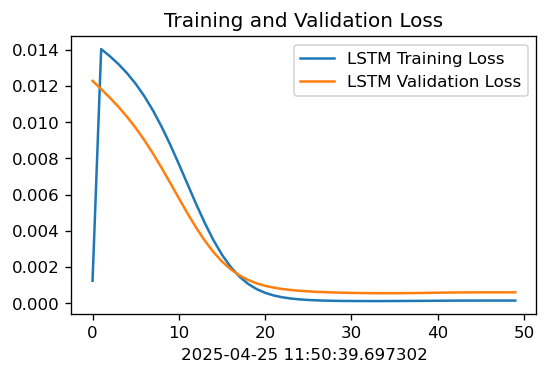

2. 调用模型进行预测

python 复制代码

predicted_y_lstm = sc.inverse_transform(model(X_test).detach().numpy().reshape(-1,1))                    # 测试集输入模型进行预测
y_test_1         = sc.inverse_transform(y_test.reshape(-1,1))
y_test_one       = [i[0] for i in y_test_1]
predicted_y_lstm_one = [i[0] for i in predicted_y_lstm]
 
plt.figure(figsize=(5, 3),dpi=120)
# 画出真实数据和预测数据的对比曲线
plt.plot(y_test_one[:2000], color='red', label='real_temp')
plt.plot(predicted_y_lstm_one[:2000], color='blue', label='prediction')
 
plt.title('Title')
plt.xlabel('X')
plt.ylabel('Y')
plt.legend()
plt.show()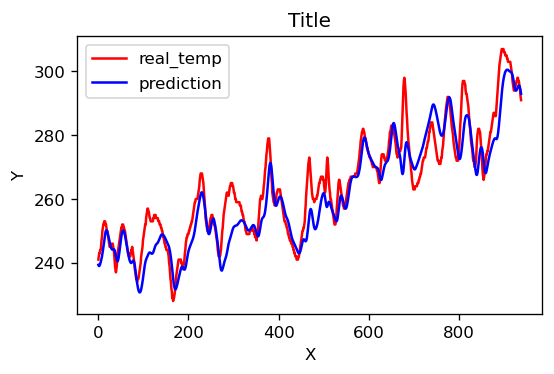

3. R2值评估

python 复制代码

from sklearn import metrics
"""
RMSE ：均方根误差  ----->  对均方误差开方
R2   ：决定系数，可以简单理解为反映模型拟合优度的重要的统计量
"""
RMSE_lstm  = metrics.mean_squared_error(predicted_y_lstm_one, y_test_1)**0.5
R2_lstm    = metrics.r2_score(predicted_y_lstm_one, y_test_1)
 
print('均方根误差: %.5f' % RMSE_lstm)
print('R2: %.5f' % R2_lstm)

均方根误差: 6.92733

R2: 0.83259

总结：

本周主要学习了LSTM模型，并且通过实践更加深入地了解到了LSTM模型。