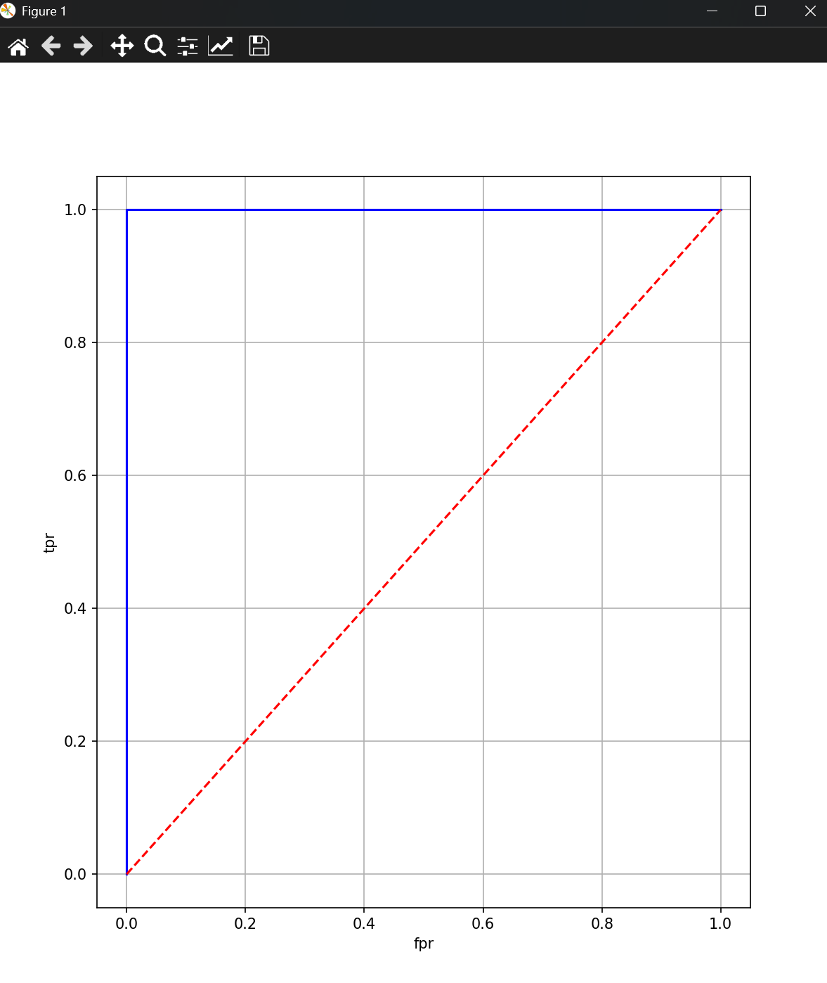
一、
题目要求:
给定以下二分类模型的预测结果,手动绘制ROC曲线并计算AUC值:
y_true = 0, 1, 0, 1, 0, 1 # 真实标签(0=负类,1=正类)
y_score = 0.2, 0.7, 0.3, 0.6, 0.1, 0.8 # 模型预测得分
代码展示:
python
import matplotlib.pyplot as plt
from sklearn.metrics import roc_curve

y_true = [0,1,0,1,0,1]
y_score = [0.2,0.7,0.3,0.6,0.1,0.8]

fpr,tpr,_ = roc_curve(y_true,y_score)

plt.figure(figsize=(8,9))
plt.plot(fpr,tpr,color="b")
plt.plot([0,1],[0,1],color="r",linestyle="--")
plt.xlabel("fpr")
plt.ylabel("tpr")
plt.grid()
plt.show()
结果展示:
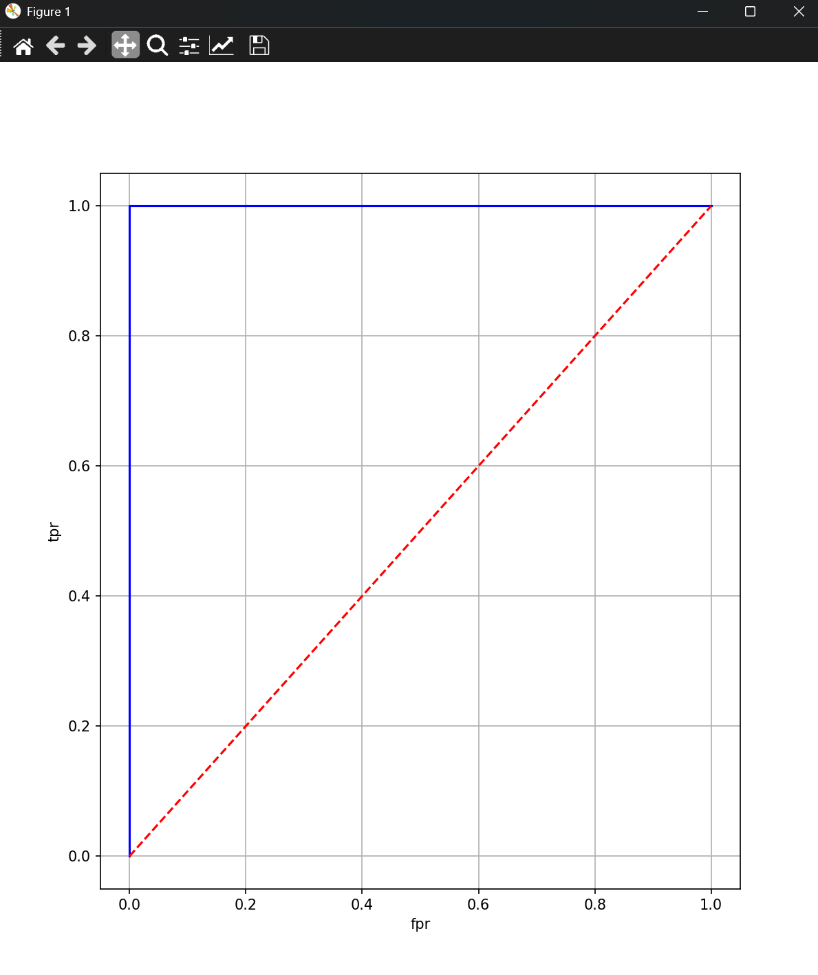
二、
题目要求
处理有相同预测得分的情况:
y_true = 1, 0, 0, 1, 1, 0, 1, 0
y_score = 0.8, 0.5, 0.5, 0.7, 0.6, 0.5, 0.9, 0.3
代码展示:
python
import matplotlib.pyplot as plt
from sklearn.metrics import roc_curve

y_true = [1, 0, 0, 1, 1, 0, 1, 0]
y_score = [0.8, 0.5, 0.5, 0.7, 0.6, 0.5, 0.9, 0.3]

fpr,tpr,_ = roc_curve(y_true,y_score)

plt.figure(figsize=(8,9))
plt.plot(fpr,tpr,color="b")
plt.plot([0,1],[0,1],color="r",linestyle="--")
plt.xlabel("fpr")
plt.ylabel("tpr")
plt.grid()
plt.show()
结果展示:
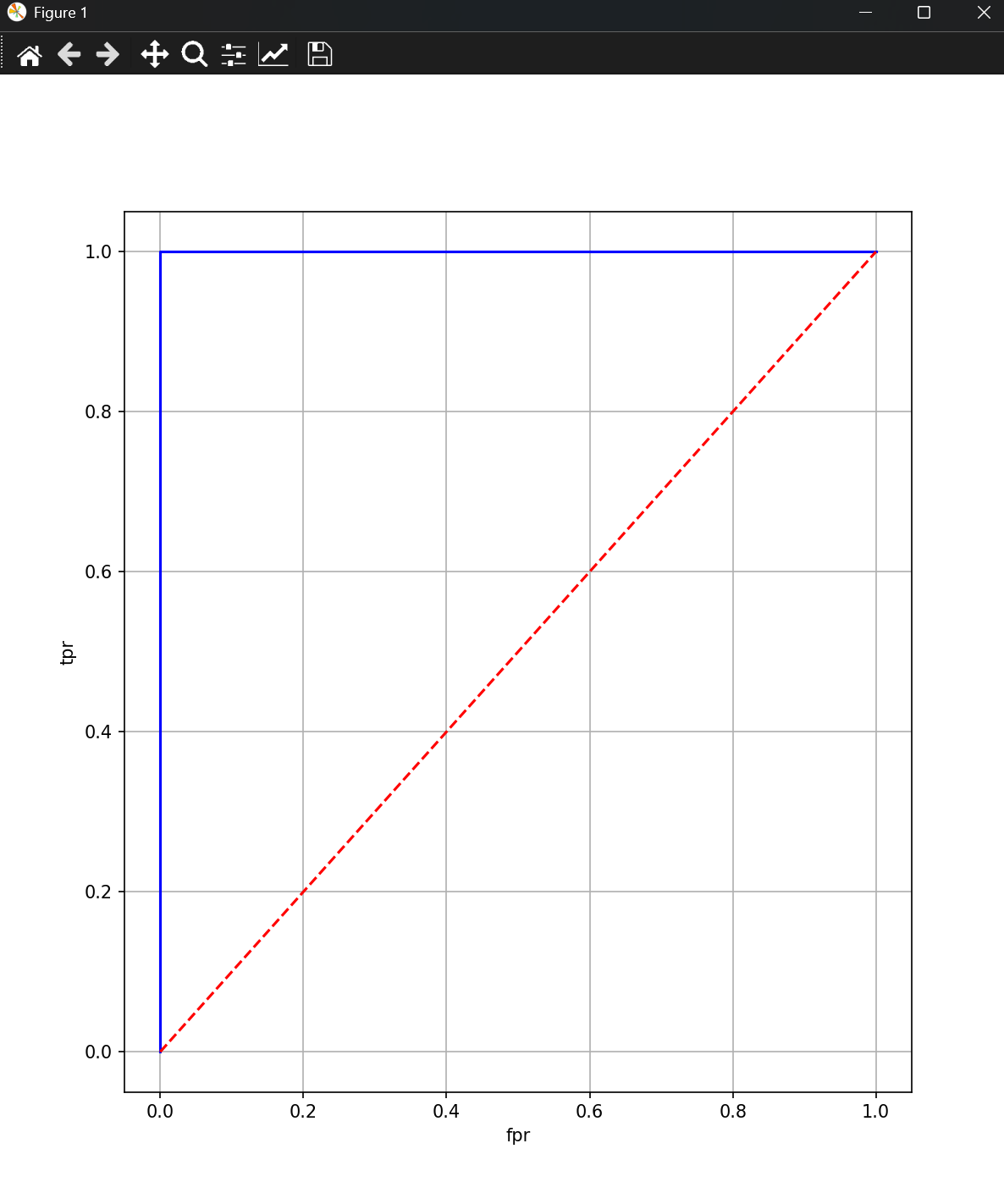
三、
题目背景
在信用卡欺诈检测中,正常交易(负类)远多于欺诈交易(正类)。给定以下模拟数据:
y_true = 0, 0, 0, 0, 0, 0, 1, 0, 1, 0 # 2个欺诈(正类),8个正常(负类)
y_score = 0.1, 0.2, 0.15, 0.05, 0.3, 0.25, 0.9, 0.4, 0.6, 0.1 # 模型输出的欺诈概率
题目要求
- 手动计算所有(FPR, TPR)点
- 绘制ROC曲线
- 观察类别不平衡对曲线形状的影响
代码展示:
python
import matplotlib.pyplot as plt
from sklearn.metrics import roc_curve

y_true = [0, 0, 0, 0, 0, 0, 1, 0, 1, 0]  # 2个欺诈(正类),8个正常(负类)
y_score = [0.1, 0.2, 0.15, 0.05, 0.3, 0.25, 0.9, 0.4, 0.6, 0.1]  # 模型输出的欺诈概率

fpr,tpr,_ = roc_curve(y_true,y_score)

plt.figure(figsize=(8,9))
plt.plot(fpr,tpr,color="b")
plt.plot([0,1],[0,1],color="r",linestyle="--")
plt.xlabel("fpr")
plt.ylabel("tpr")
plt.grid()
plt.show()
结果展示:
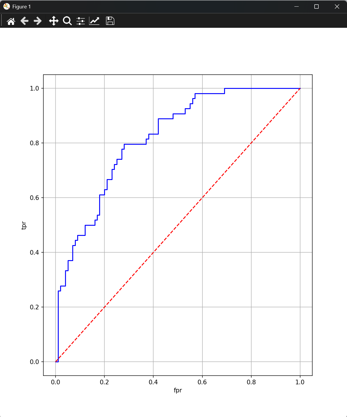
四、
使用Kaggle上的"Pima Indians Diabetes Database"数据集来进行逻辑回归的练习。该数据集的链接如下:Pima Indians Diabetes Database
练习场景描述:
你是一家医疗机构的数据分析师,你的任务是分析Pima Indians Diabetes Database数据集,以预测患者是否患有糖尿病。数据集包含了一系列与患者健康相关的指标,如怀孕次数、葡萄糖浓度、血压等。你需要使用逻辑回归模型来训练一个分类器,以根据这些指标预测患者是否患有糖尿病。
具体步骤:
- 使用pandas库加载数据集,并进行初步的数据探索,了解数据集的字段和分布情况。
- 对数据进行预处理,包括处理缺失值、标准化或归一化特征值等。
- 使用numpy库进行特征选择或特征工程,以提高模型的性能。
- 划分训练集和测试集,使用训练集训练逻辑回归模型,并使用测试集评估模型的性能。
- 使用matplotlib库绘制ROC曲线或混淆矩阵,以直观展示模型的分类效果。
- 根据评估结果调整模型的参数,以提高模型的性能。
题目:
基于上述练习场景,请完成以下任务:
- 加载Pima Indians Diabetes Database数据集,并进行初步的数据探索。
- 对数据进行预处理,包括处理缺失值和标准化特征值。
- 使用逻辑回归模型进行训练,并评估模型的性能。
- 绘制ROC曲线,展示模型的分类效果。
- 根据你的理解,提出至少一个改进模型性能的方法,并尝试实现。
代码展示:
python
import matplotlib.pyplot as plt
import pandas as pd
from sklearn.linear_model import LogisticRegression
from sklearn.metrics import roc_curve
from sklearn.model_selection import train_test_split, GridSearchCV
from sklearn.preprocessing import StandardScaler

df = pd.read_csv("./data/diabetes.csv",encoding="utf-8")
print(df.head())
print(df.shape)

df = df.dropna(axis=0)

x = df.drop("Outcome",axis=1)
y = df["Outcome"]

x_train,x_test,y_train,y_test = train_test_split(x,y,test_size=0.2,random_state=22)

transfer = StandardScaler()
x_train = transfer.fit_transform(x_train)
x_test = transfer.fit_transform(x_test)

estimator = LogisticRegression()
estimator.fit(x_train,y_train)

y_predict = estimator.predict(x_test)
print("预测值和真实的对比:",y_predict == y_test)

ret = estimator.score(x_test,y_test)
print("准确率:",ret)

y_pred_proba = estimator.predict_proba(x_test)[:, 1]
fpr, tpr, thresholds = roc_curve(y_test, y_pred_proba)

plt.figure(figsize=(8,9))
plt.plot(fpr,tpr,color="b")
plt.plot([0,1],[0,1],color="r",linestyle="--")
plt.xlabel("fpr")
plt.ylabel("tpr")
plt.grid()
plt.show()

param_grid = {
    'C': [0.1, 1, 10, 100],
    'penalty': ['l1', 'l2'],
    'solver': ['liblinear', 'saga']
}
grid_search = GridSearchCV(LogisticRegression(), param_grid, cv=5)
grid_search.fit(x_train, y_train)

best_estimator = grid_search.best_estimator_
best_ret = best_estimator.score(x_test, y_test)
print("调整参数后模型的准确率:", best_ret)
结果展示:
python
预测值和真实的对比: 645    False
767     True
31      True
148    False
59      True
       ...
30      True
158     True
167     True
582    False
681     True
Name: Outcome, Length: 154, dtype: bool
准确率: 0.7402597402597403
调整参数后模型的准确率: 0.7402597402597403