(a)
yield <-data.frame(
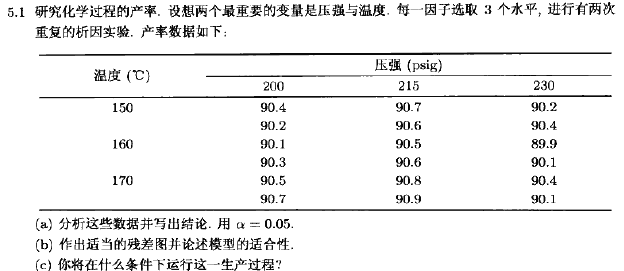
X = c(90.4,90.2,90.7,90.6,90.2,90.4,90.1,90.3,90.5,90.6,89.9,90.1,90.5,90.7,90.8,90.9,90.4,90.1),
A = gl(3, 2,18), #pressure (A ) and temperature (B)
B = gl(3, 6, 18)
)
yield.aov<-aov(X~A*B, data=yield )
> summary(yield.aov)
Df Sum Sq Mean Sq F value Pr(>F)
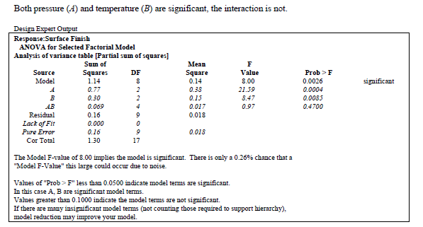
A 2 0.7678 0.3839 21.594 0.000367 ***
B 2 0.3011 0.1506 8.469 0.008539 **
A:B 4 0.0689 0.0172 0.969 0.470006
Residuals 9 0.1600 0.0178
Signif. codes:
0 '***' 0.001 '**' 0.01 '*' 0.05 '.' 0.1 ' ' 1
bartlett.test(X~A, data=batter) # 对因素A
bartlett.test(X~B, data=batter) #对因素B
fit <-lm(X~A*B,data=yield)
anova(fit)
> anova(fit)
Analysis of Variance Table
Response: X
Df Sum Sq Mean Sq F value Pr(>F)
A 2 0.76778 0.38389 21.5937 0.0003673 ***
B 2 0.30111 0.15056 8.4687 0.0085392 **
A:B 4 0.06889 0.01722 0.9687 0.4700058
Residuals 9 0.16000 0.01778
Signif. codes:
0 '***' 0.001 '**' 0.01 '*' 0.05 '.' 0.1 ' ' 1
summary(fit)
> summary(fit)
Call:
lm(formula = X ~ A * B, data = yield)
Residuals:
Min 1Q Median 3Q Max
-0.15 -0.10 0.00 0.10 0.15
Coefficients:
Estimate Std. Error t value Pr(>|t|)
(Intercept) 9.030e+01 9.428e-02 957.776 <2e-16
A2 3.500e-01 1.333e-01 2.625 0.0276
A3 -7.480e-14 1.333e-01 0.000 1.0000
B2 -1.000e-01 1.333e-01 -0.750 0.4724
B3 3.000e-01 1.333e-01 2.250 0.0510
A2:B2 8.190e-14 1.886e-01 0.000 1.0000
A3:B2 -2.000e-01 1.886e-01 -1.061 0.3165
A2:B3 -1.000e-01 1.886e-01 -0.530 0.6087
A3:B3 -3.500e-01 1.886e-01 -1.856 0.0964
(Intercept) ***
A2 *
A3
B2
B3 .
A2:B2
A3:B2
A2:B3
A3:B3 .
Signif. codes:
0 '***' 0.001 '**' 0.01 '*' 0.05 '.' 0.1 ' ' 1
Residual standard error: 0.1333 on 9 degrees of freedom
Multiple R-squared: 0.8767, Adjusted R-squared: 0.7671
F-statistic: 8 on 8 and 9 DF, p-value: 0.002638
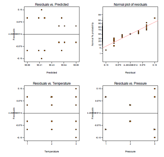
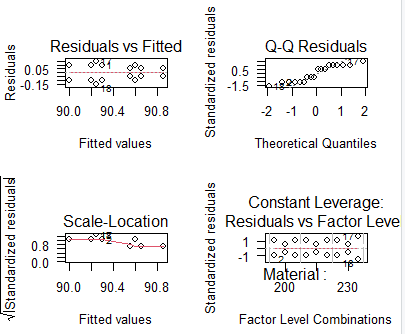
par(mfrow=c(2,2))
plot(fit)
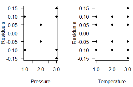
par(mfrow=c(1,2))
plot(as.numeric(yieldA), fitresiduals, xlab="Pressure", ylab="Residuals", type="p", pch=16)
plot(as.numeric(yieldB), fitresiduals, xlab="Temperature", ylab="Residuals", pch=16)
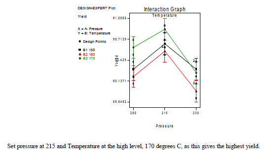
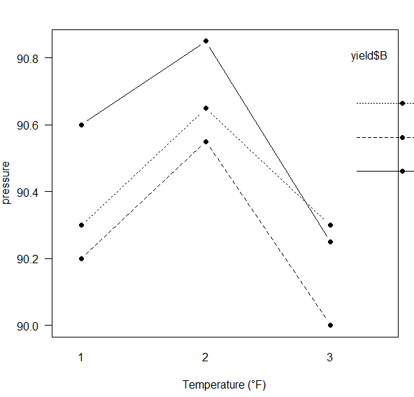
with(battery,interaction.plot(yieldA,yieldB,yield$X,type="b",pch=19,fixed=T,xlab="Temperature (°F)",ylab="pressure"))
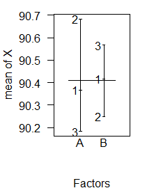
plot.design(X~A*B,data=yield)
yield <-data.frame(
X = c(90.4,90.2,90.7,90.6,90.2,90.4,90.1,90.3,90.5,90.6,89.9,90.1,90.5,90.7,90.8,90.9,90.4,90.1),
A = c(150,150,150,150,150,150,160,160,160,160,160,160,170,170,170,170,170,170), #pressure (A ) and temperature (B)
B = c(200,200,215,215,230,230,200,200,215,215,230,230,200,200,215,215,230,230)
)
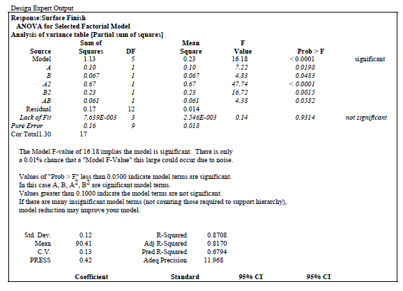
fit <-lm(X~A*B+I(A^2)*I(B^2)+A:I(B^2)+B:I(A^2),data=yield)
anova(fit)
summary(fit)
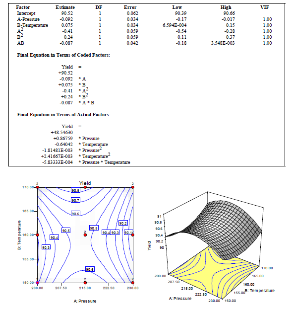
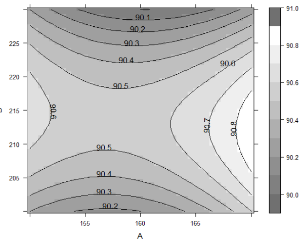
tmp.B <- seq(200,230,by=.5)
tmp.A <- seq(150,170,by=.5)
tmp <- list(A=tmp.A,B=tmp.B)
new <- expand.grid(tmp)
new$fit <- c(predict(fit,new))
require(lattice)
contourplot (fit~A*B ,data=new, cuts=8,region=T,col.regions=gray(7:16/16))
yield <-data.frame(
X = c(90.4,90.2,90.7,90.6,90.2,90.4,90.1,90.3,90.5,90.6,89.9,90.1,90.5,90.7,90.8,90.9,90.4,90.1),
B = gl(3, 2,18), #pressure (A ) and temperature (B)
A = gl(3, 6, 18)
)
fit <-lm(as.numeric(X)~as.numeric(A)*as.numeric(B)+I(as.numeric(A)^2)*I(as.numeric(B)^2)+A:I(as.numeric(B)^2)+as.numeric(B):I(as.numeric(A)^2),data=yield)
anova(fit)
summary(fit)
tmp.A <- seq(200,230,by=.5)
tmp.B <- seq(150,170,by=.5)
tmp <- list(A=tmp.A,B=tmp.B)
new <- expand.grid(tmp)
new$fit <- c(predict(fit,new))
require(lattice)
contourplot (fit~A*B ,data=new, cuts=8,region=T,col.regions=gray(7:16/16))