【数据可视化】2023 年 Spotify 歌曲数据集可视化分析

🧑 博主简介：曾任某智慧城市类企业算法总监，CSDN / 稀土掘金等平台人工智能领域优质创作者。
目前在美国市场的物流公司从事高级算法工程师一职，深耕人工智能领域，精通python数据挖掘、可视化、机器学习等，发表过AI相关的专利并多次在AI类比赛中获奖。

一、引言

在当今音乐流媒体蓬勃发展的时代，数据分析对于音乐产业的决策制定至关重要。本文将利用2023年Spotify歌曲数据集，从多个维度进行可视化分析，深入探讨影响歌曲流行度和音频特征的关键因素。该数据集涵盖了丰富的信息，包括歌曲名称、艺术家姓名、流媒体统计数据和音频特征等，为音乐分析师和研究人员提供了宝贵的数据支持。以下分析将使用Matplotlib库实现，提供完整的代码示例，以供读者参考和复现。

二、数据探索

2.1 数据集介绍

2023年Spotify歌曲数据集包含以下变量：

track_name：歌曲名称
artist(s)_name：艺术家姓名
artist_count：参与歌曲创作的艺术家数量
released_year：歌曲发行年份
released_month：歌曲发行月份
released_day：歌曲发行日
in_spotify_playlists：歌曲包含在Spotify播放列表中的数量
in_spotify_charts：歌曲在Spotify排行榜中的位置和是否存在
streams：Spotify上的总播放次数
in_apple_playlists：歌曲包含在Apple Music播放列表中的数量
in_apple_charts：歌曲在Apple Music排行榜中的位置和是否存在
in_deezer_playlists：歌曲包含在Deezer播放列表中的数量
in_deezer_charts：歌曲在Deezer排行榜中的位置和是否存在
in_shazam_charts：歌曲在Shazam排行榜中的位置和是否存在
bpm：每分钟节拍数，衡量歌曲的节奏速度
key：歌曲的调式
mode：歌曲的调式（大调或小调）
danceability_% ：歌曲适合跳舞的百分比
valence_% ：歌曲音乐内容的积极性百分比
energy_% ：歌曲的感知能量水平百分比
acousticness_% ：歌曲中的原声音频部分的百分比
instrumentalness_% ：歌曲中的器乐内容的百分比
liveness_% ：歌曲中现场表演元素的存在百分比
speechiness_% ：歌曲中口语单词的百分比

2.2 数据清洗探索

python 复制代码

import pandas as pd
import numpy as np
import matplotlib.pyplot as plt

# 加载数据
df = pd.read_csv('spotify_songs_2023.csv', encoding='latin1')  # 请替换为实际文件路径

# 查看数据基本信息
df.shape
print(df.info())
print(df.isna().sum())
# 将发布日期列转换为日期类型
df['released_date'] = pd.to_datetime(df[['released_year', 'released_month', 'released_day']].apply(lambda x: f"{x['released_year']}-{x['released_month']}-{x['released_day']}", axis=1), errors='coerce')

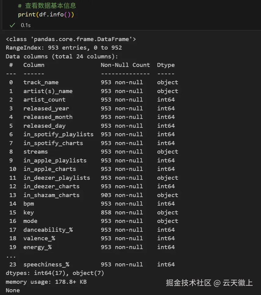
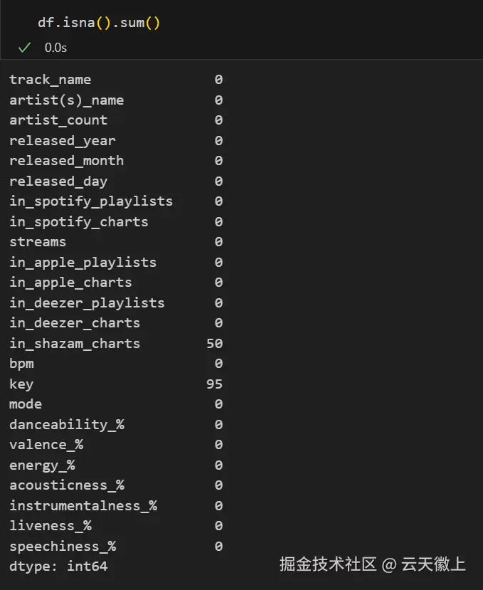
从数据基本信息可发现：

数据共24个维度，包含字符串和数值类型。
部分特征可能存在缺失值，需进一步清洗。

三、单维度特征可视化

3.1 歌曲发行年份分布

python 复制代码

plt.figure(figsize=(10, 6))
plt.hist(df['released_year'].dropna(), bins=10, color='skyblue', edgecolor='black')
plt.title('Song Release Year Distribution')
plt.xlabel('Year')
plt.ylabel('Count')
plt.grid(axis='y')
plt.show()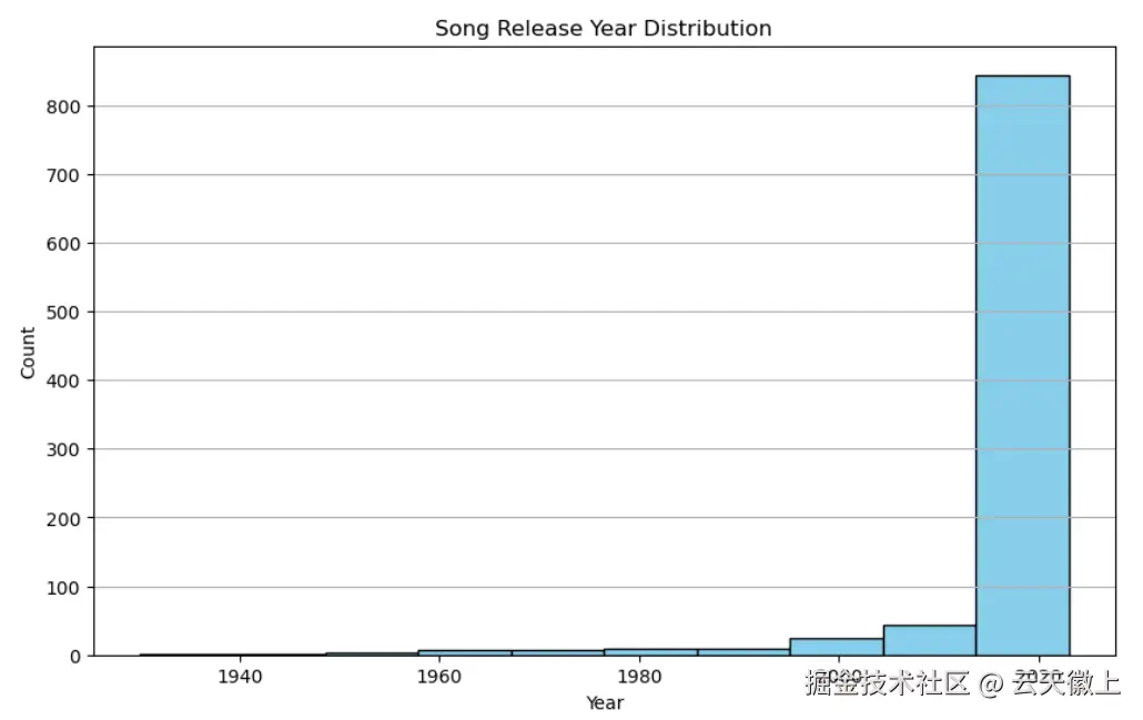

3.2 艺术家数量分布

python 复制代码

plt.figure(figsize=(8, 6))
plt.hist(df['artist_count'], bins=10, color='lightgreen', edgecolor='black')
plt.title('Artist Count Distribution')
plt.xlabel('Number of Artists')
plt.ylabel('Count')
plt.grid(axis='y')
plt.show()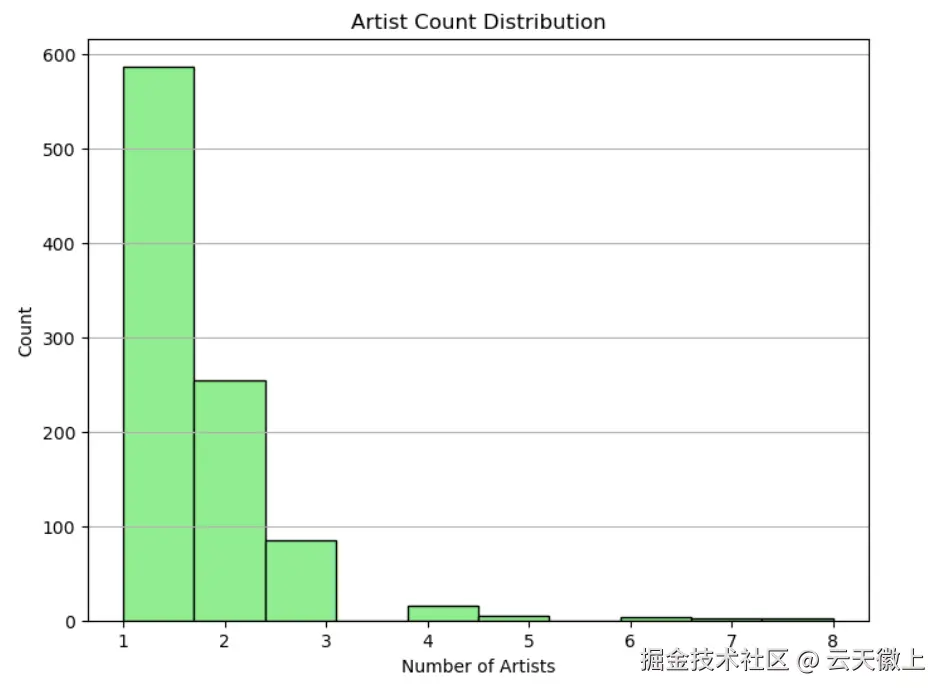

3.3 歌曲在Spotify播放列表中的分布

python 复制代码

plt.figure(figsize=(10, 6))
plt.hist(df['in_spotify_playlists'], bins=20, color='lightcoral', edgecolor='black')
plt.title('Spotify Playlists Distribution')
plt.xlabel('Number of Playlists')
plt.ylabel('Count')
plt.grid(axis='y')
plt.show()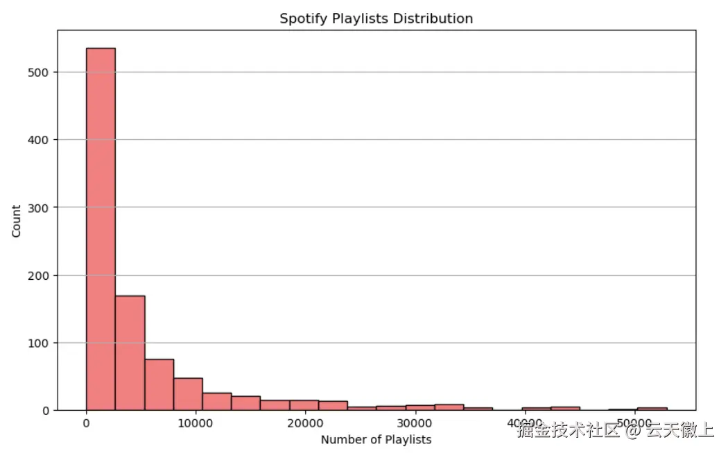

3.4 歌曲在Spotify排行榜中的分布

python 复制代码

plt.figure(figsize=(10, 6))
plt.hist(df['in_spotify_charts'].dropna(), bins=10, color='gold', edgecolor='black')
plt.title('Spotify Charts Distribution')
plt.xlabel('Chart Rank')
plt.ylabel('Count')
plt.grid(axis='y')
plt.show()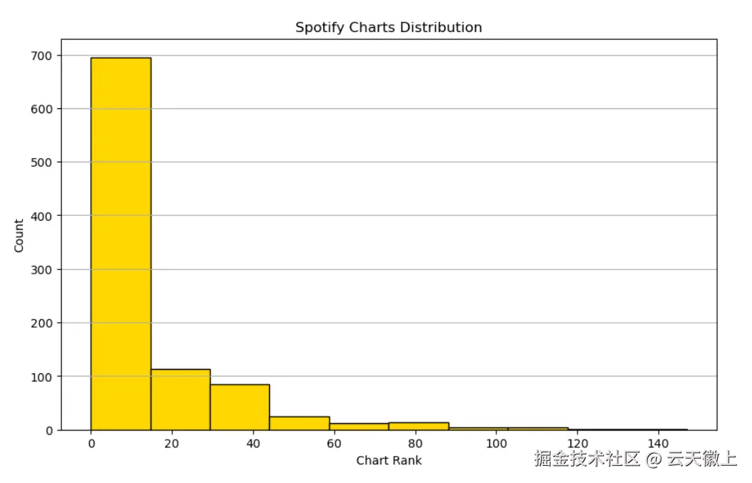

3.5 歌曲播放次数分布

python 复制代码

plt.figure(figsize=(10, 6))
df['streams'] = df['streams'].apply(lambda x:int(x) if x.isdigit() else None)
plt.hist(df['streams'], bins=20, color='lightblue', edgecolor='black')
plt.title('Streams Distribution')
plt.xlabel('Number of Streams')
plt.ylabel('Count')
plt.grid(axis='y')
plt.show()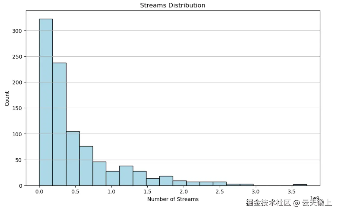

四、各个特征与歌曲流行度关系的可视化

4.1 节拍速度（BPM）与播放次数关系

python 复制代码

plt.figure(figsize=(10, 6))
plt.scatter(df['bpm'], df['streams'], alpha=0.5, color='purple')
plt.title('BPM vs Streams')
plt.xlabel('BPM')
plt.ylabel('Streams')
plt.grid(True)
plt.show()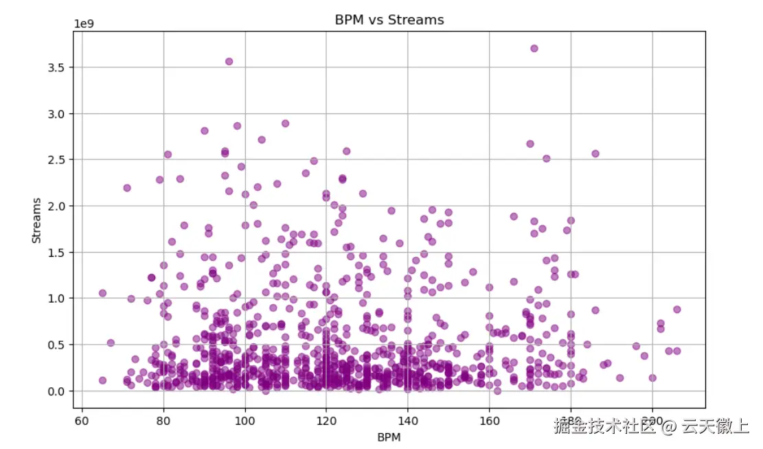

4.2 调式与播放次数关系

python 复制代码

df = df.dropna(axis=0, subset=['streams'])#丢弃datetime和values这两列中有缺失值的行
plt.figure(figsize=(8, 6))
plt.boxplot([df[df['mode'] == 'Major']['streams'].tolist(), df[df['mode'] == 'Minor']['streams'].tolist()], labels=['Major', 'Minor'])
plt.title('Streams by Mode')
plt.ylabel('Streams')
plt.grid(True)
plt.show()

4.3 可舞性与播放次数关系

python 复制代码

plt.figure(figsize=(10, 6))
plt.scatter(df['danceability_%'], df['streams'], alpha=0.5, color='lightgreen')
plt.title('Danceability vs Streams')
plt.xlabel('Danceability (%)')
plt.ylabel('Streams')
plt.grid(True)
plt.show()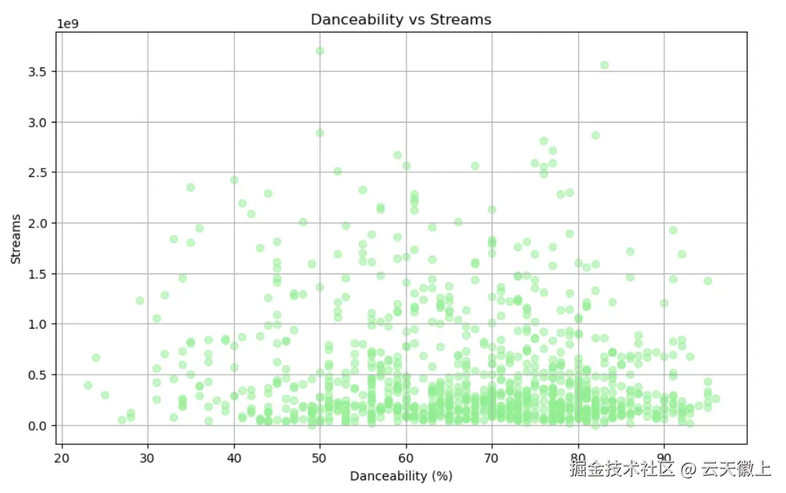

4.4 歌曲能量与播放次数关系

python 复制代码

plt.figure(figsize=(10, 6))
plt.scatter(df['energy_%'], df['streams'], alpha=0.5, color='skyblue')
plt.title('Energy vs Streams')
plt.xlabel('Energy (%)')
plt.ylabel('Streams')
plt.grid(True)
plt.show()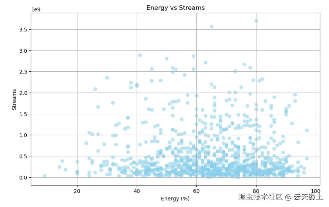

4.5 多维度组合分析（调式、可舞性与播放次数）

python 复制代码

plt.figure(figsize=(12, 6))
for mode in df['mode'].unique():
    subset = df[df['mode'] == mode]
    plt.scatter(subset['danceability_%'], subset['streams'], label=mode, alpha=0.5)
plt.title('Streams vs Danceability by Mode')
plt.xlabel('Danceability (%)')
plt.ylabel('Streams')
plt.legend()
plt.grid(True)
plt.show()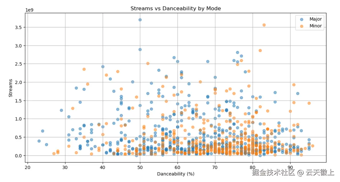

4.6 多维度组合分析（调式、能量与播放次数）

python 复制代码

plt.figure(figsize=(12, 6))
for mode in df['mode'].unique():
    subset = df[df['mode'] == mode]
    plt.scatter(subset['energy_%'], subset['streams'], label=mode, alpha=0.5)
plt.title('Streams vs Energy by Mode')
plt.xlabel('Energy (%)')
plt.ylabel('Streams')
plt.legend()
plt.grid(True)
plt.show()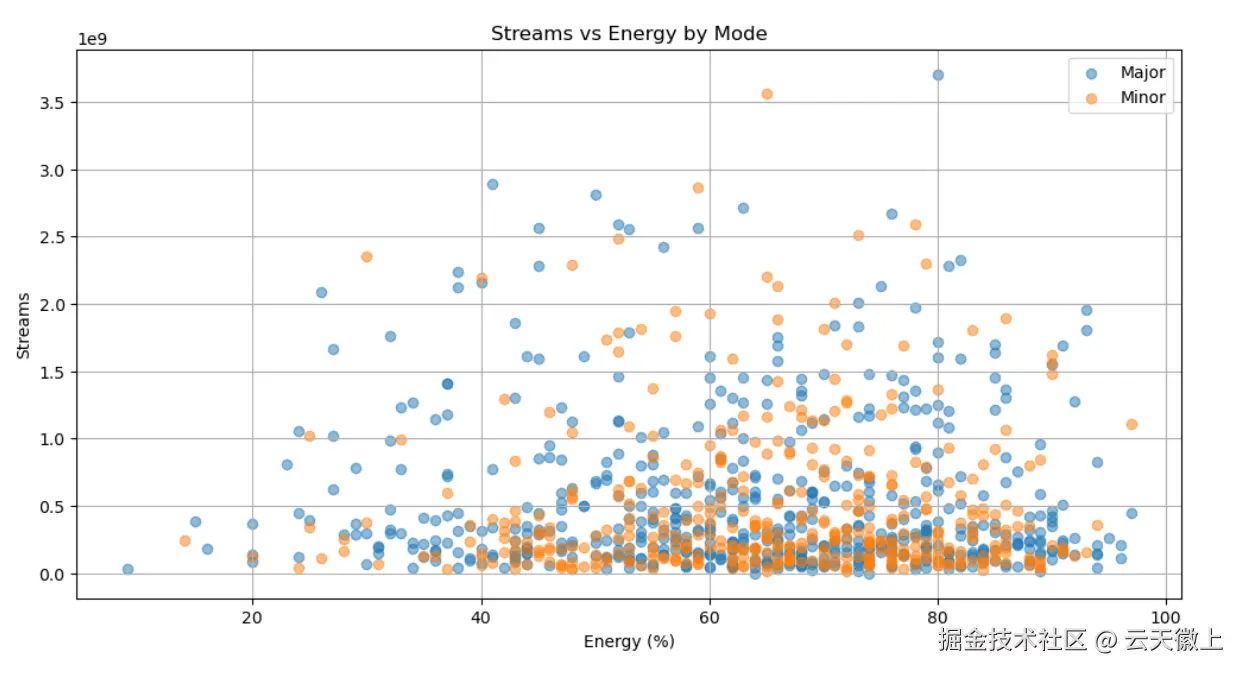

4.7 歌曲在不同平台播放列表中的分布

python 复制代码

plt.figure(figsize=(12, 8))
platforms = ['Spotify', 'Apple Music', 'Deezer']
metrics = ['in_spotify_playlists', 'in_apple_playlists', 'in_deezer_playlists']
colors = ['skyblue', 'lightgreen', 'lightcoral']

for i, (platform, metric) in enumerate(zip(platforms, metrics)):
    plt.subplot(3, 1, i + 1)
    plt.hist(df[metric], bins=20, color=colors[i], edgecolor='black')
    plt.title(f'{platform} Playlists Distribution')
    plt.xlabel('Number of Playlists')
    plt.ylabel('Count')
    plt.grid(axis='y')

plt.tight_layout()
plt.show()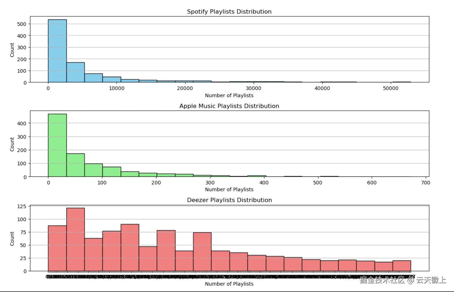

4.8 歌曲在不同平台排行榜中的分布

python 复制代码

plt.figure(figsize=(12, 8))
platforms = ['Spotify', 'Apple Music', 'Deezer', 'Shazam']
metrics = ['in_spotify_charts', 'in_apple_charts', 'in_deezer_charts', 'in_shazam_charts']

for i, (platform, metric) in enumerate(zip(platforms, metrics)):
    plt.subplot(4, 1, i + 1)
    plt.hist(df[metric].dropna(), bins=10, color=plt.cm.tab20(i), edgecolor='black')
    plt.title(f'{platform} Charts Distribution')
    plt.xlabel('Chart Rank')
    plt.ylabel('Count')
    plt.grid(axis='y')

plt.tight_layout()
plt.show()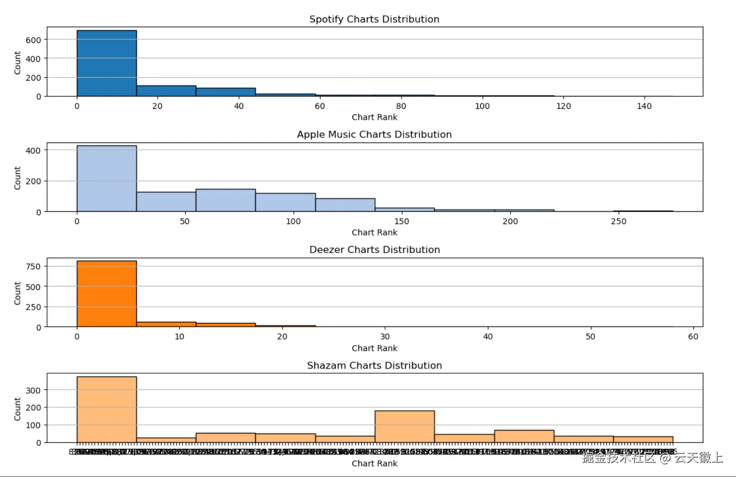

4.9 歌曲音频特征组合分析

python 复制代码

plt.figure(figsize=(12, 8))
audio_features = ['danceability_%', 'valence_%', 'energy_%', 'acousticness_%', 'instrumentalness_%', 'liveness_%', 'speechiness_%']
colors = ['skyblue', 'lightgreen', 'lightcoral', 'gold', 'purple', 'lightblue', 'lightgreen']

for i, feature in enumerate(audio_features):
    plt.subplot(4, 2, i + 1)
    plt.hist(df[feature], bins=20, color=colors[i % len(colors)], edgecolor='black')
    plt.title(f'{feature.replace("_", " ").title()} Distribution')
    plt.xlabel(feature.replace("_", " ").title())
    plt.ylabel('Count')
    plt.grid(axis='y')

plt.tight_layout()
plt.show()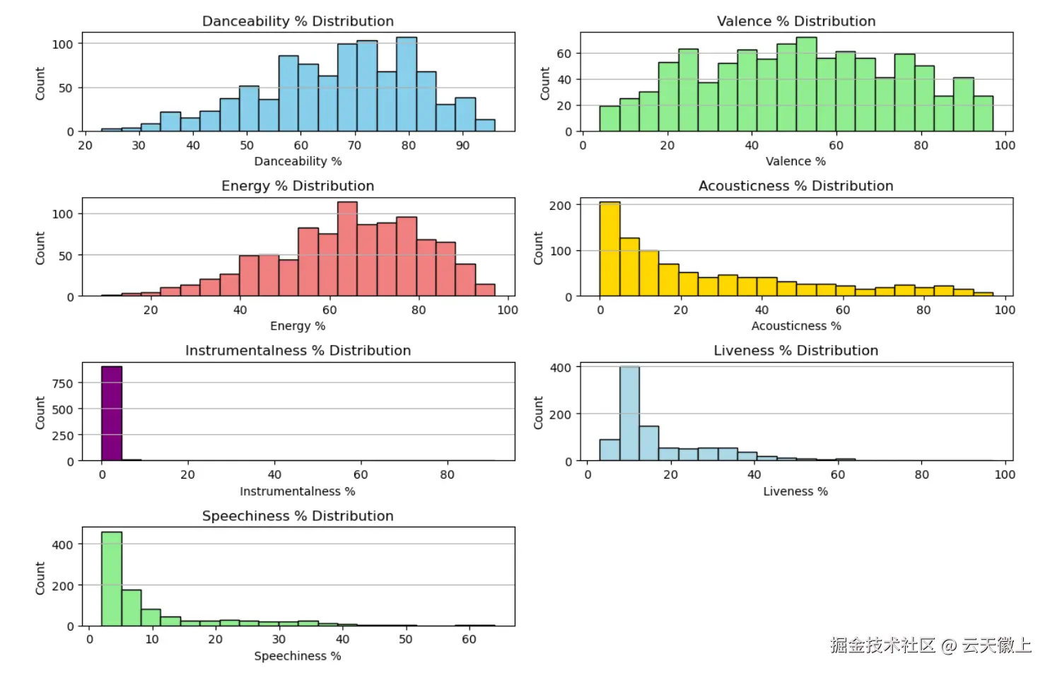

4.10 多维度组合分析（调式、可舞性、能量与播放次数）

python 复制代码

plt.figure(figsize=(14, 10))
modes = df['mode'].unique()
danceability_ranges = [0, 25, 50, 75, 100]
danceability_labels = ['Low', 'Medium-Low', 'Medium-High', 'High']

for i, mode in enumerate(modes):
    plt.subplot(2, 2, i + 1)
    subset = df[df['mode'] == mode]
    subset['Danceability Range'] = pd.cut(subset['danceability_%'], bins=danceability_ranges, labels=danceability_labels)
    for j, energy_range in enumerate(danceability_labels):
        subsubset = subset[subset['Danceability Range'] == energy_range]
        plt.scatter(subsubset['energy_%'], subsubset['streams'], label=energy_range, alpha=0.5)
    plt.title(f'Streams vs Energy by Danceability Range ({mode})')
    plt.xlabel('Energy (%)')
    plt.ylabel('Streams')
    plt.legend()
    plt.grid(True)

plt.tight_layout()
plt.show()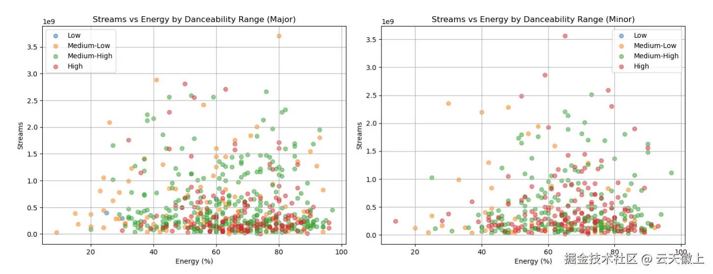

4.11 多维度组合分析（调式、能量、可舞性与播放次数）

python 复制代码

plt.figure(figsize=(14, 10))
modes = df['mode'].unique()
energy_ranges = [0, 25, 50, 75, 100]
energy_labels = ['Low', 'Medium-Low', 'Medium-High', 'High']

for i, mode in enumerate(modes):
    plt.subplot(2, 2, i + 1)
    subset = df[df['mode'] == mode]
    subset['Energy Range'] = pd.cut(subset['energy_%'], bins=energy_ranges, labels=energy_labels)
    for j, energy_label in enumerate(energy_labels):
        subsubset = subset[subset['Energy Range'] == energy_label]
        plt.scatter(subsubset['danceability_%'], subsubset['streams'], label=energy_label, alpha=0.5)
    plt.title(f'Streams vs Danceability by Energy Range ({mode})')
    plt.xlabel('Danceability (%)')
    plt.ylabel('Streams')
    plt.legend()
    plt.grid(True)

plt.tight_layout()
plt.show()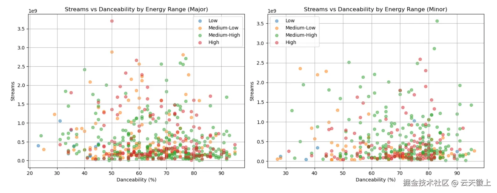

从以上可视化分析可以看出：

歌曲发行年份分布：歌曲发行年份集中在近几年，反映了数据集的时效性。
艺术家数量分布：大多数歌曲由单个或少数几个艺术家合作完成。
歌曲在Spotify播放列表中的分布：少数歌曲被大量播放列表收录，表明其受欢迎程度。
歌曲在Spotify排行榜中的分布：排名靠前的歌曲数量较少，头部效应明显。
歌曲播放次数分布：播放次数呈现长尾分布，少数歌曲获得极高播放量。
节拍速度与播放次数关系：中等节奏的歌曲通常获得较高的播放量。
调式与播放次数关系：大调歌曲通常比小调歌曲更受欢迎。
可舞性与播放次数关系：可舞性较高的歌曲通常获得更多的播放量。
歌曲能量与播放次数关系：高能量歌曲通常更受听众欢迎。
多维度组合分析：不同调式、可舞性和能量组合对歌曲流行度的影响显著，反映了听众对音乐风格的偏好。

以上分析为音乐分析师和研究人员提供了多维度视角，揭示了影响歌曲流行度和音频特征的关键因素，为音乐创作和推广策略提供了数据支持。

**注：**博主目前收集了6900+份相关数据集，有想要的可以领取部分数据：

如果您在人工智能领域遇到技术难题，或是需要专业支持，无论是技术咨询、项目开发还是个性化解决方案，我都可以为您提供专业服务，如有需要可站内私信或添加下方VX名片（ID：xf982831907）

期待与您一起交流，共同探索AI的更多可能！