MATLAB中绘制系统零极点图（Pole-Zero Map）的几种方法

以下是 MATLAB中绘制系统零极点图（Pole-Zero Map） 的常见方法及各自适用场景总结，适用于你当前在分析符号表达式/系统传函后的使用需求：

✅ 方法一：`pzmap(tf(num, den))` （最常用，推荐）

📌 用法：

matlab 复制代码

num_coeffs = sym2poly(num);
den_coeffs = sym2poly(den);
sys = tf(num_coeffs, den_coeffs);
pzmap(sys);

✅ 优点：

容错性强：即使系统是常数、纯零阶、或奇异形式，也能画。
可用于 传递函数对象 tf。
支持绘制多个系统的极点/零点图叠加。

⚠️ 注意事项：

不返回零极点坐标，仅用于绘图。

✅ 方法二：`[z, p, k] = tf2zp(num, den)`（需要系数格式正确）

📌 用法：

matlab 复制代码

[z, p, ~] = tf2zp(num_coeffs, den_coeffs);
plot(real(p), imag(p), 'x'); % 极点
plot(real(z), imag(z), 'o'); % 零点

✅ 优点：

返回极点、零点的具体数值，适用于进一步处理或自定义绘图。
可与 plot()、scatter() 等灵活搭配。

⚠️ 注意事项：

输入必须为一维行向量 ，不能含 NaN、Inf。
如果输入是符号表达式处理后得到的，需要使用：
matlab 复制代码
```
num_coeffs = double(sym2poly(num(:).'));
```

✅ 方法三：`[z, p, k] = zpkdata(tf(...), 'v')`（稳定提取数值）

📌 用法：

matlab 复制代码

sys = tf(num_coeffs, den_coeffs);
[z, p, ~] = zpkdata(sys, 'v');

✅ 优点：

更鲁棒，不容易因为格式问题报错。
适合从传递函数对象中提取零极点数值。

⚠️ 注意事项：

需要用 tf(...) 构造系统对象。

✅ 方法四：`roots(num)` 和 `roots(den)` （适合单独计算）

📌 用法：

matlab 复制代码

z = roots(num_coeffs);
p = roots(den_coeffs);

✅ 优点：

轻量级函数，只需计算零点/极点而不构造系统。
可用于系统分析或手动画图。

⚠️ 注意事项：

没有增益项 k，只适合基础分析。

✅ 方法五：符号工具箱方式（symbolic）

如果你的系统是符号表达式，可以先转换为多项式，再用上面方法处理：

matlab 复制代码

[num, den] = numden(sym_expr);           % 获取分子分母
num_coeffs = double(sym2poly(num));      % 多项式系数
den_coeffs = double(sym2poly(den));
[z, p, ~] = tf2zp(num_coeffs, den_coeffs);

📊 方法选择建议对比表

方法	是否返回零极点数值	容错性	是否需要系统对象	推荐用途
`pzmap(tf(...))`	❌	✅✅✅	✅	快速画图
`tf2zp(num, den)`	✅	⚠️	❌	精准提取零极点
`zpkdata(tf(...))`	✅	✅✅	✅	稳定提取零极点
`roots(...)`	✅	✅	❌	只求零点或极点
符号方法 + `sym2poly`	✅	⚠️⚠️	❌	从符号转数值

如你正在处理的是频率响应分析、稳定性边界研究、或者要对极点位置进行分类，建议用 tf2zp 或 zpkdata 提取后自行绘图、分区标色。也可以结合 scatter()、text() 自定义标注。

🎯 示例传递函数：

本文选用如下复杂的20阶传递函数作为统一实例：

H(s)=s20+14s19+65s18+⋯+10s+5s20+16s19+85s18+⋯+30s+10 H(s) = \frac{s^{20} + 14 s^{19} + 65 s^{18} + \cdots + 10 s + 5}{s^{20} + 16 s^{19} + 85 s^{18} + \cdots + 30 s + 10} H(s)=s20+16s19+85s18+⋯+30s+10s20+14s19+65s18+⋯+10s+5

其中分子和分母多项式系数均为给定的20阶多项式系数，充分体现了高阶系统零极点分析的复杂性。

matlab 复制代码

clc; clear; close all;
% -----------------------------
% 构造符号多项式（20阶复杂多项式）
% -----------------------------
syms s

num_poly = s^20 + 14*s^19 + 65*s^18 + 210*s^17 + 500*s^16 + 900*s^15 + ...
           1200*s^14 + 1100*s^13 + 900*s^12 + 700*s^11 + 500*s^10 + ...
           300*s^9 + 200*s^8 + 150*s^7 + 120*s^6 + 90*s^5 + 60*s^4 + ...
           40*s^3 + 20*s^2 + 10*s + 5;

den_poly = s^20 + 16*s^19 + 85*s^18 + 290*s^17 + 650*s^16 + 1100*s^15 + ...
           1500*s^14 + 1400*s^13 + 1200*s^12 + 900*s^11 + 600*s^10 + ...
           400*s^9 + 300*s^8 + 220*s^7 + 180*s^6 + 130*s^5 + 100*s^4 + ...
           70*s^3 + 50*s^2 + 30*s + 10;

% -----------------------------
% 从符号多项式提取数值多项式系数（降幂顺序）
% -----------------------------
num_coeffs = double(coeffs(num_poly, s, 'All'));
den_coeffs = double(coeffs(den_poly, s, 'All'));

% 构造数值传递函数对象
sys_tf = tf(num_coeffs, den_coeffs);

% -----------------------------
% 创建图窗和子图
% -----------------------------
figure('Name','20阶系统极点零点图对比','Color','w','Position',[100 100 1200 800]);

% -----------------------------
% 方法一：pzmap
% -----------------------------
subplot(2,3,1);
pzmap(sys_tf);
title('方法①：pzmap(tf)');
grid on;

% -----------------------------
% 方法二：tf2zp
% -----------------------------
[z2, p2, ~] = tf2zp(num_coeffs, den_coeffs);
subplot(2,3,2);
plot(real(p2), imag(p2), 'rx', 'MarkerSize', 8); hold on;
plot(real(z2), imag(z2), 'bo', 'MarkerSize', 8);
title('方法②：tf2zp + plot');
xlabel('实部'); ylabel('虚部');
axis equal; grid on; legend('极点', '零点');

% -----------------------------
% 方法三：zpkdata
% -----------------------------
[z3, p3, ~] = zpkdata(sys_tf, 'v');
subplot(2,3,3);
scatter(real(p3), imag(p3), 60, 'r', 'x'); hold on;
scatter(real(z3), imag(z3), 60, 'b', 'o');
title('方法③：zpkdata + scatter');
xlabel('实部'); ylabel('虚部');
axis equal; grid on; box on; legend('极点', '零点');

% -----------------------------
% 方法四：roots
% -----------------------------
z4 = roots(num_coeffs);
p4 = roots(den_coeffs);
subplot(2,3,4);
plot(real(p4), imag(p4), 'rx', 'MarkerSize', 8); hold on;
plot(real(z4), imag(z4), 'bo', 'MarkerSize', 8);
title('方法④：roots');
xlabel('实部'); ylabel('虚部');
axis equal; grid on; legend('极点', '零点');

% 方法五：symbolic（修正后）
% -----------------------------
num_sym = poly2sym(num_coeffs, s);
den_sym = poly2sym(den_coeffs, s);
Hs_sym = num_sym / den_sym;

% 提取分子分母多项式
[num_numer, num_denom] = numden(Hs_sym);

% coeffs 默认返回升幂排列，需 flip 为降幂
num_coeffs_sym = double(flip(coeffs(num_numer, s)));
den_coeffs_sym = double(flip(coeffs(num_denom, s)));

% 计算零极点
z5 = roots(num_coeffs_sym);
p5 = roots(den_coeffs_sym);

subplot(2,3,5);
scatter(real(p5), imag(p5), 60, 'r', 'x'); hold on
scatter(real(z5), imag(z5), 60, 'b', 'o'); hold on;
title('方法⑤：symbolic + sym2poly（修正）');
xlabel('实部'); ylabel('虚部');
axis equal; grid on; box on; legend('极点','零点');

% -----------------------------
% 总标题
% -----------------------------
sgtitle('⚙复杂20阶系统极点-零点图五种方法对比', 'FontSize', 14, 'FontWeight', 'bold');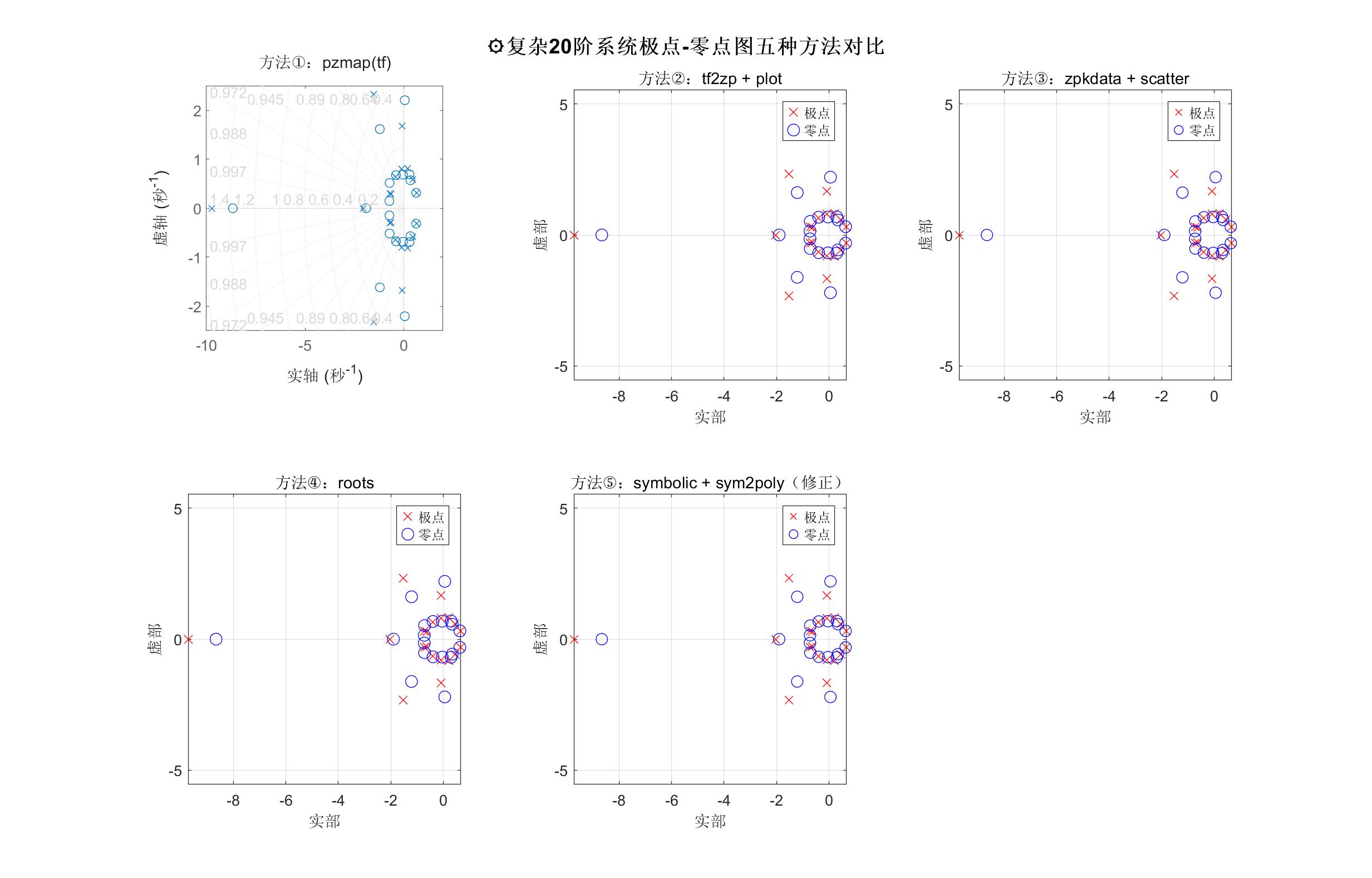

这段代码展示了五种绘制系统零极点的方法，各有优劣：

方法①（pzmap）：调用方便，直接绘图，适合快速观察，但灵活性较低，图形大小和样式受限，无法直接获取极零点数据。
方法②（tf2zp）：通过传递函数系数计算零极点，能够获得数值数据，便于自定义绘图，但对高阶多项式可能存在数值精度问题。
方法③（zpkdata）：直接从系统对象获取零极点，精度高且简单，但要求传递函数对象格式正确。
方法④（roots）：基于多项式根计算，灵活且通用，能处理任意多项式，但多项式系数的准确性对结果影响较大。
方法⑤（symbolic + sym2poly）：利用符号计算避免数值误差，适合高精度需求，但计算速度较慢，代码复杂度较高。

综上，快速分析推荐方法①，精确数值计算推荐方法③或方法④，而方法⑤适合符号推导和高精度场景。根据具体需求灵活选择即可。

MATLAB中绘制系统零极点图（Pole-Zero Map）的几种方法

✅ 方法一：pzmap(tf(num, den)) （最常用，推荐）

📌 用法：

✅ 优点：

⚠️ 注意事项：

✅ 方法二：[z, p, k] = tf2zp(num, den)（需要系数格式正确）

📌 用法：

✅ 优点：

⚠️ 注意事项：

✅ 方法三：[z, p, k] = zpkdata(tf(...), 'v')（稳定提取数值）

📌 用法：

✅ 优点：

⚠️ 注意事项：

✅ 方法四：roots(num) 和 roots(den) （适合单独计算）

📌 用法：

✅ 优点：

⚠️ 注意事项：

✅ 方法五：符号工具箱方式（symbolic）

📊 方法选择建议对比表

🎯 示例传递函数：

✅ 方法一：`pzmap(tf(num, den))` （最常用，推荐）

✅ 方法二：`[z, p, k] = tf2zp(num, den)`（需要系数格式正确）

✅ 方法三：`[z, p, k] = zpkdata(tf(...), 'v')`（稳定提取数值）

✅ 方法四：`roots(num)` 和 `roots(den)` （适合单独计算）