遥感&机器学习入门实战教程｜Sklearn 案例④ ：多分类器对比（SVM / RF / kNN / Logistic...）

在前几篇文章中，我们已经学习了 无泄露 PCA 的降维流程，以及如何在单个分类器上实现整图预测。今天我们进一步扩展：

👉 使用 多个分类器（SVM、RF、kNN、Logistic、AdaBoost） 对比精度

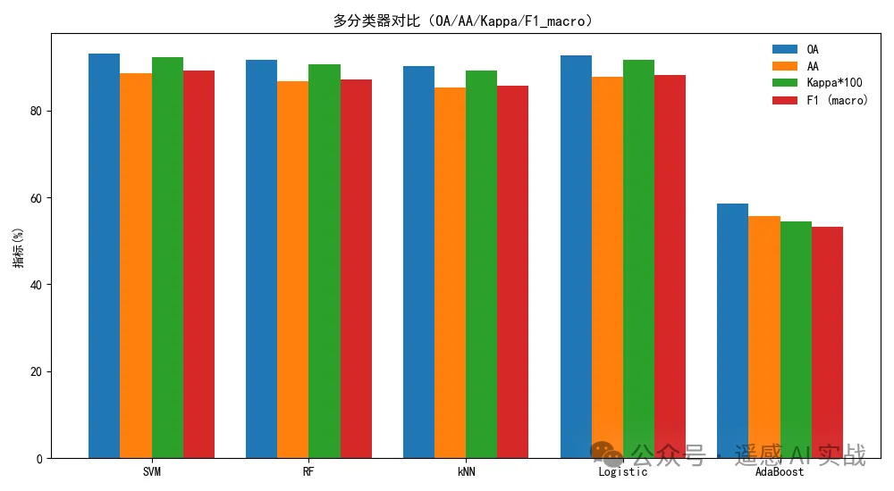
👉 给出 OA / AA / Kappa 三个指标的对比条形图

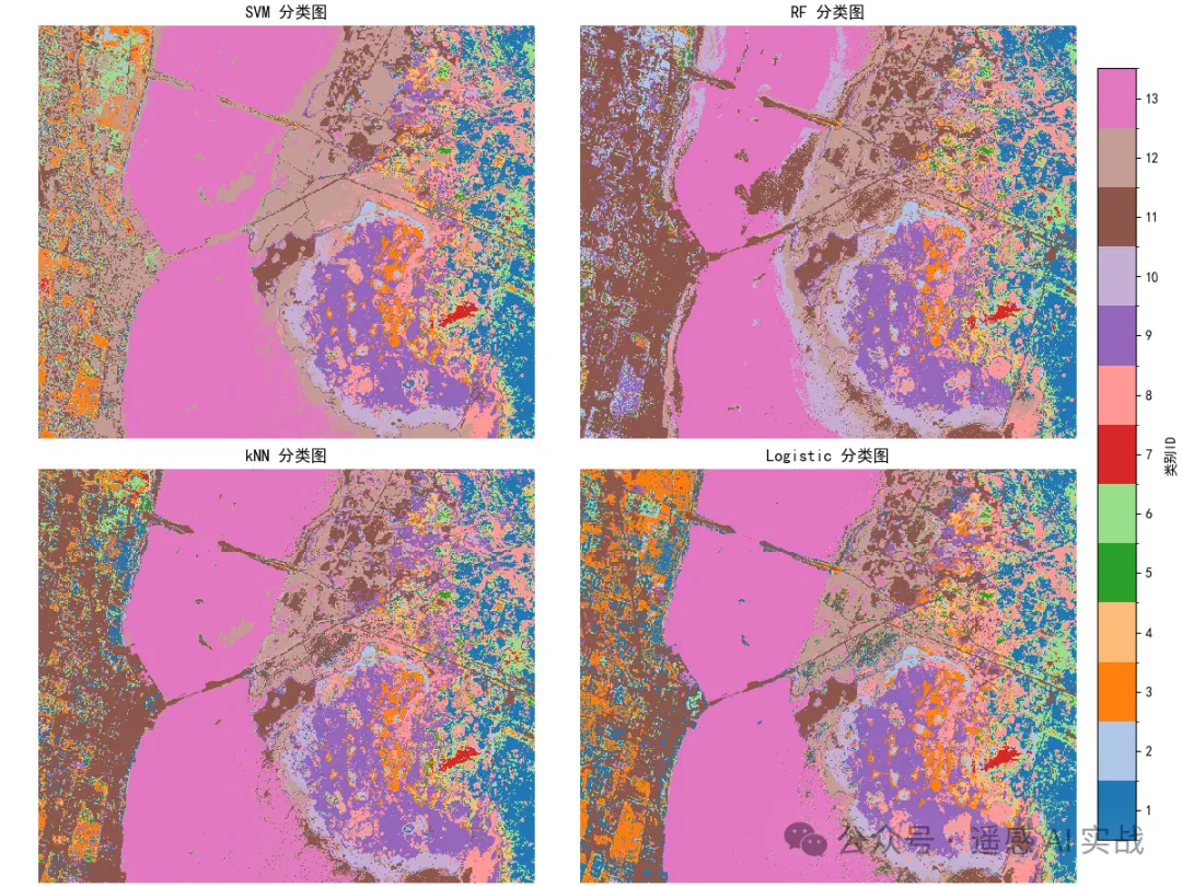
👉 新增 整图预测可视化，通过 2×2 子图直观展示不同分类器在整幅影像上的预测结果差异

数据与任务

我们使用 KSC 高光谱影像 (KSC.mat) 及其地物标注 (KSC_gt.mat)。完成：

• StandardScaler 标准化 + PCA 降维（只用训练集 fit，再对整图 transform）
• 五类经典分类器（SVM、随机森林、kNN、Logistic、AdaBoost）对比
• 指标：OA / AA / Kappa / F1（macro）
• 整图预测的 2×2 可视化（SVM / RF / kNN / Logistic）

1) 环境与全局参数

Sklearn 亮点：

• train_test_split 支持 stratify 分层抽样；
• StandardScaler/PCA 是常见的"先标准化、再降维"预处理管道；
• 设定随机种子有助于复现实验。

# 1) 依赖与参数
import os, time
import numpy as np
import scipy.io as sio
import matplotlib.pyplot as plt

from sklearn.model_selection import train_test_split
from sklearn.preprocessing import StandardScaler
from sklearn.decomposition import PCA
from sklearn.svm import SVC
from sklearn.ensemble import RandomForestClassifier, AdaBoostClassifier
from sklearn.neighbors import KNeighborsClassifier
from sklearn.linear_model import LogisticRegression
from sklearn.metrics import (confusion_matrix, classification_report,
                             accuracy_score, cohen_kappa_score, f1_score)

# ===== 修改为你的数据路径（包含 KSC.mat 与 KSC_gt.mat）=====
DATA_DIR = r"your_path"

# 实验参数
PCA_DIM = 30
TRAIN_RATIO = 0.3
SEED = 42

2) 读取与抽取有标注像素

Sklearn 亮点：本段暂不调用算法；目的是把数据整理成 sklearn 善用的"样本×特征"二维表。

# 2) 加载 KSC 影像与标注
X = sio.loadmat(os.path.join(DATA_DIR, "KSC.mat"))["KSC"].astype(np.float32)   # (H, W, B)
Y = sio.loadmat(os.path.join(DATA_DIR, "KSC_gt.mat"))["KSC_gt"].astype(int)    # (H, W)

h, w, b = X.shape
coords = np.argwhere(Y != 0)                 # 有标签像素的坐标
labels = Y[coords[:, 0], coords[:, 1]] - 1   # 0-based 标签（sklearn 常用）
num_classes = int(labels.max() + 1)

print(f"H×W×Bands = {h}×{w}×{b}, labeled={len(coords)}, classes={num_classes}")

3) 分层划分训练/测试集

Sklearn 亮点：

• train_test_split(..., stratify=labels) 让每个类别在 train/test 中"成分相似"。
• 这一步只在有标签像素上进行。

# 3) 分层抽样划分
train_ids, test_ids = train_test_split(
    np.arange(len(coords)),
    train_size=TRAIN_RATIO,
    stratify=labels,
    random_state=SEED
)

print(f"train={len(train_ids)}, test={len(test_ids)}")

4) 无泄露预处理：StandardScaler + PCA

Sklearn 使用：

• StandardScaler().fit(训练像素)：只在训练集 fit，避免把测试信息泄露进数据分布；
• PCA(n_components=PCA_DIM)：在标准化之后做降维；
• 对整图先 reshape 成 (H*W, B)，再 transform，最后还原形状。

# 4) 仅用训练像素拟合 StandardScaler 与 PCA
train_pixels = X[coords[train_ids, 0], coords[train_ids, 1]]  # (N_train, B)

scaler = StandardScaler().fit(train_pixels)                                   # 只用训练集 fit
pca    = PCA(n_components=PCA_DIM, random_state=SEED).fit(scaler.transform(train_pixels))

# 整图统一 transform（不会泄露）
X_flat      = X.reshape(-1, b)
X_std       = scaler.transform(X_flat)
X_pca_flat  = pca.transform(X_std)
X_pca       = X_pca_flat.reshape(h, w, PCA_DIM)

# 从降维后的整图中抽样训练/测试像素
X_train = X_pca[coords[train_ids, 0], coords[train_ids, 1]]
y_train = labels[train_ids]
X_test  = X_pca[coords[test_ids, 0],  coords[test_ids, 1]]
y_test  = labels[test_ids]

print("X_train:", X_train.shape, "X_test:", X_test.shape)

5) 定义五类经典分类器

Sklearn 使用（核心参数）：

• SVC(kernel='rbf', C, gamma)：

  • C 越大越"重罚误分"（可能过拟合），gamma 控制 RBF 核宽度（越大越"窄"）；

• RandomForestClassifier(n_estimators, max_depth)：

  • 多棵随机树投票，n_estimators 越多越稳但更慢；

• KNeighborsClassifier(n_neighbors, weights)：

  • weights='distance' 常比等权投票更稳；

• LogisticRegression(solver='lbfgs', max_iter)：

  • 多类别默认为"multinomial"，max_iter 需足够大保证收敛；

• AdaBoostClassifier(n_estimators)：

  • 迭代强调难分类样本的权重，适合弱学习器提升。

# 5) 五类模型
models = {
    "SVM":      SVC(kernel="rbf", C=20, gamma=0.005),
    "RF":       RandomForestClassifier(n_estimators=400, max_depth=20, random_state=SEED, n_jobs=-1),
    "kNN":      KNeighborsClassifier(n_neighbors=5, weights="distance", n_jobs=-1),
    "Logistic": LogisticRegression(max_iter=2000, tol=1e-4, solver="lbfgs"),   # 不显式设置 multi_class（>=1.5 已默认 multinomial）
    "AdaBoost": AdaBoostClassifier(n_estimators=200, random_state=SEED)
}

6) 训练与评估（OA / AA / Kappa / F1）

Sklearn 使用：

• classification_report 一次给出 per-class Precision/Recall/F1；
• accuracy_score = OA；
• AA（Average Accuracy） 可理解为召回的宏平均 ：np.mean(diag(cm)/row_sum)；
• cohen_kappa_score 衡量与随机一致性的改进；
• f1_score(..., average='macro') 得到宏平均 F1。

# 6) 训练与评估
results = {}
y_preds = {}   # 留作后续整图预测/对比

for name, clf in models.items():
    clf.fit(X_train, y_train)
    y_pred = clf.predict(X_test)
    y_preds[name] = y_pred

    # 基础指标
    oa     = accuracy_score(y_test, y_pred)
    kappa  = cohen_kappa_score(y_test, y_pred)
    cm     = confusion_matrix(y_test, y_pred, labels=np.arange(num_classes))
    aa     = float(np.nanmean(np.diag(cm) / np.maximum(cm.sum(axis=1), 1)))
    f1m    = f1_score(y_test, y_pred, average='macro')

    results[name] = {"OA": oa, "AA": aa, "Kappa": kappa, "F1_macro": f1m}

    print(f"\n=== {name} ===")
    print(f"OA={oa*100:.2f}%  AA={aa*100:.2f}%  Kappa={kappa:.4f}  F1_macro={f1m*100:.2f}%")
    print(classification_report(y_test, y_pred, digits=4))

---

7) 指标横向对比条形图

Sklearn 使用 ：评价指标都在 sklearn.metrics 里；这里我们把 OA/AA/Kappa/F1 宏平均绘到同一张图上，更直观。

# 7) 可视化对比
labels_plot = ["SVM", "RF", "kNN", "Logistic", "AdaBoost"]
oa_vals     = [results[m]["OA"]*100       for m in labels_plot]
aa_vals     = [results[m]["AA"]*100       for m in labels_plot]
kappa_vals  = [results[m]["Kappa"]*100    for m in labels_plot]
f1_vals     = [results[m]["F1_macro"]*100 for m in labels_plot]

x = np.arange(len(labels_plot))
width = 0.2

plt.figure(figsize=(10, 5.5))
plt.bar(x - 1.5*width, oa_vals,    width, label="OA")
plt.bar(x - 0.5*width, aa_vals,    width, label="AA")
plt.bar(x + 0.5*width, kappa_vals, width, label="Kappa*100")
plt.bar(x + 1.5*width, f1_vals,    width, label="F1 (macro)")
plt.xticks(x, labels_plot)
plt.ylabel("指标(%)")
plt.title("多分类器对比（OA/AA/Kappa/F1_macro）")
plt.legend(frameon=False)
plt.tight_layout()
plt.show()

8) 整图预测（2×2 子图对比：SVM / RF / kNN / Logistic）

Sklearn 使用：

• 训练好的 estimator 可直接对 (H*W, PCA_DIM) 的整图特征进行 predict；
• matplotlib 配合 BoundaryNorm 把色标做成离散类别，避免"连续 colormap"的误导；
• constrained_layout=True 自动处理子图与 colorbar 布局，不会互相遮挡。

# 8) 整图预测与 2×2 对比
from matplotlib.colors import ListedColormap, BoundaryNorm

# 只展示四个模型（可按需扩展）
show_keys = ["SVM", "RF", "kNN", "Logistic"]

# 每个模型的整图预测（类别改为 1..C 便于阅读）
pred_maps = {}
for key in show_keys:
    pred = models[key].predict(X_pca_flat)        # (H*W,)
    pred_maps[key] = pred.reshape(h, w) + 1       # (H, W), 1..C

# 统一调色板（离散类别对齐到整数刻度）
base_cmap  = plt.get_cmap('tab20')
colors     = [base_cmap(i % 20) for i in range(num_classes)]
cmap       = ListedColormap(colors)
boundaries = np.arange(0.5, num_classes + 1.5, 1)
norm       = BoundaryNorm(boundaries, cmap.N)

fig, axes = plt.subplots(2, 2, figsize=(12, 9), constrained_layout=True)
axes = axes.ravel()

ims = []
for ax, key in zip(axes, show_keys):
    im = ax.imshow(pred_maps[key], cmap=cmap, norm=norm, interpolation='nearest')
    ax.set_title(f"{key} 分类图", fontsize=12)
    ax.axis('off')
    ims.append(im)

# 共享一个总色条，离散刻度；适当抽稀刻度避免过密
cbar = fig.colorbar(
    ims[0],
    ax=axes.tolist(),
    location='right',
    shrink=0.9,
    pad=0.02,
    boundaries=boundaries,
    ticks=np.arange(1, num_classes + 1, max(1, num_classes // 12))
)
cbar.set_label("类别ID", rotation=90)
plt.show()

结果展示

精度结果：

在前几篇文章中，我们已经学习了 无泄露 PCA 的降维流程，以及如何在单个分类器上实现整图预测。

今天我们进一步扩展：

👉 使用 多个分类器（SVM、RF、kNN、Logistic、AdaBoost） 对比精度

👉 给出 OA / AA / Kappa 三个指标的对比条形图

👉 新增 整图预测可视化，通过 2×2 子图直观展示不同分类器在整幅影像上的预测结果差异

分类图：

进一步思考

• SVM 参数里，C 与 gamma 十分关键：若你想系统搜索，建议使用 GridSearchCV 或 HalvingGridSearchCV。
• 随机森林 的 feature_importances_ 可帮助理解哪些主成分（或波段组合）更重要。
• kNN 对距离度量敏感，标准化与降维往往显著提升效果。
• Logistic 若仍提示收敛，可增大 max_iter 或将 solver='saga'（更适合大样本或带正则化的场景）。
• AdaBoost 默认基学习器是 DecisionTreeClassifier(max_depth=1)（桩树），也可替换为更强的弱学习器（注意计算代价与过拟合）。

你现在可以做的扩展

1. 在本框架中加入 混淆矩阵可视化（计数/归一化两版）以定位"易混类"。
2. 引入 交叉验证 进行参数搜索，并把 cv_results_ 绘成热力图（第③篇已示范）。
3. 使用 Voting/Stacking 把多个模型组合起来（可作为第五篇主题）。

欢迎大家关注下方我的公众获取更多内容！