一、Conv2D 介绍
Conv2D 是一种专门用于处理二维数据(如图像、音频频谱)的卷积层。它通过滑动卷积核(滤波器)在输入图像上进行卷积操作,从而提取局部特征。与一维卷积(Conv1D)不同,Conv2D 在两个维度上进行卷积,适合处理图像、音频频谱等数据。
1.1 Conv2D 的结构与参数
结构
- 输入层 :二维输入数据,通常为形状为
(batch_size, in_channels, height, width)的张量。 - 卷积层 :包含多个卷积核,每个卷积核的大小为
(kernel_height, kernel_width),用于提取特征。 - 激活层:通常使用 ReLU 激活函数,引入非线性。
参数
- in_channels:输入数据的通道数(例如,对于 RGB 图像,通道数为 3)。
- out_channels :卷积层输出的通道数,即卷积核的数量。
- kernel_size:卷积核的大小,可以是单个整数(如 3)或一个元组(如 (3, 5))。
- stride:步幅,卷积核在输入图像上滑动的步长,默认为 1。
- padding:填充方式,可以是 'valid'(无填充)或 'same'(填充以保持输出大小与输入相同)。
- dilation:卷积核元素之间的间距,默认为 1。用于扩张卷积。
- groups:控制输入和输出通道之间的连接方式。默认为 1,表示所有通道都连接。
权重
在 Conv2D 中,卷积核的权重是可学习的参数。每个卷积核的权重会在训练过程中通过反向传播算法进行更新。具体来说:
- 权重矩阵 :对于每个卷积核,权重矩阵的形状为
(in_channels, kernel_height, kernel_width)。整个 Conv2D 权重矩阵的形状为(out_channels, in_channels, kernel_height, kernel_width)。 - 偏置项 :每个卷积核都有一个独立的偏置项,用于调整该卷积核的输出。整个 Conv2D 偏置项的形状为
(out_channels,),其中out_channels是卷积核的数量。
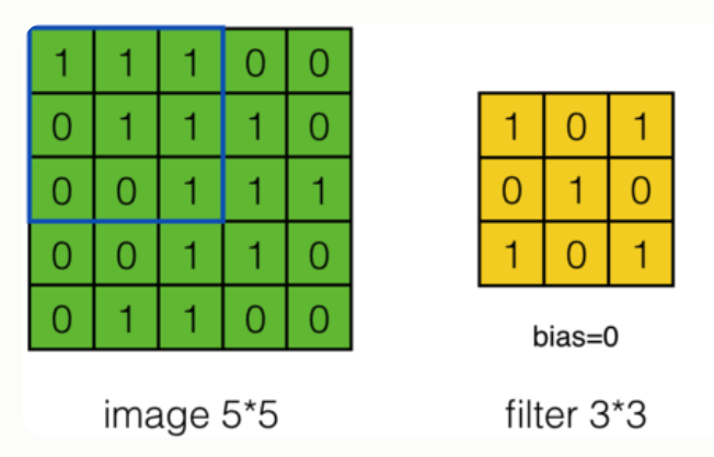
计算过程
在卷积操作中,卷积核的权重与输入数据的对应区域进行逐元素相乘,然后求和,得到一个输出值。
单通道情况:
Yi,j=∑m=0kh−1∑n=0kw−1Xi+m,j+n⋅Wm,n+bYi, j = \sum_{m=0}^{k_h-1} \sum_{n=0}^{k_w-1} Xi+m, j+n \cdot Wm, n + bYi,j=m=0∑kh−1n=0∑kw−1Xi+m,j+n⋅Wm,n+b
其中:
- Yi,jYi, jYi,j:输出特征图在位置(i,j)(i, j)(i,j)的值
- XXX:输入图像
- WWW:卷积核权重
- bbb:偏置项
- khk_hkh 和 kwk_wkw:卷积核的高度和宽度
多通道情况:
Yc,i,j=bc+∑d=0Cin−1∑m=0kh−1∑n=0kw−1Xd,i+m,j+n⋅Wc,d,m,nYc, i, j = bc + \sum_{d=0}^{C_{in}-1} \sum_{m=0}^{k_h-1} \sum_{n=0}^{k_w-1} Xd, i+m, j+n \cdot Wc, d, m, nYc,i,j=bc+d=0∑Cin−1m=0∑kh−1n=0∑kw−1Xd,i+m,j+n⋅Wc,d,m,n
其中:
- Yc,i,jYc, i, jYc,i,j:输出特征图在通道 ccc、位置 (i,j)(i, j)(i,j) 的值
- bcbcbc:通道 c 的偏置项
- CinC_{in}Cin:输入通道数
- Xd,i+m,j+nXd, i+m, j+nXd,i+m,j+n:输入图像在通道 ddd、位置 (i+m,j+n)(i+m, j+n)(i+m,j+n) 的值
- Wc,d,m,nWc, d, m, nWc,d,m,n:卷积核在输出通道 ccc、输入通道 ddd、位置 (m,n)(m, n)(m,n) 的权重
实际计算中还需要考虑步长(stride)和填充(padding):
Yc,i,j=bc+∑d=0Cin−1∑m=0kh−1∑n=0kw−1Xpaddedd,i×sh+m,j×sw+n⋅Wc,d,m,nYc, i, j = bc + \sum_{d=0}^{C_{in}-1} \sum_{m=0}^{k_h-1} \sum_{n=0}^{k_w-1} X_{padded}d, i \\times s_h + m, j \\times s_w + n \cdot Wc, d, m, nYc,i,j=bc+d=0∑Cin−1m=0∑kh−1n=0∑kw−1Xpaddedd,i×sh+m,j×sw+n⋅Wc,d,m,n
其中:
- shs_hsh 和 sws_wsw:高度和宽度方向的步长
- XpaddedX_{padded}Xpadded:填充后的输入图像
- iii 和 jjj:输出位置索引
1.2 输入输出维度
-
输入数据维度 :
(batch_size, in_channels, height, width) -
输出数据维度 :
(batch_size, out_channels, new_height, new_width)
输出尺寸公式:
Hout=⌊Hin+2×paddingh−dilationh×(kernel_sizeh−1)−1strideh+1⌋H_{out} = \left\lfloor \frac{H_{in} + 2 \times \text{padding}_h - \text{dilation}_h \times (\text{kernel\_size}_h - 1) - 1}{\text{stride}_h} + 1 \right\rfloorHout=⌊stridehHin+2×paddingh−dilationh×(kernel_sizeh−1)−1+1⌋
Wout=⌊Win+2×paddingw−dilationw×(kernel_sizew−1)−1stridew+1⌋W_{out} = \left\lfloor \frac{W_{in} + 2 \times \text{padding}_w - \text{dilation}_w \times (\text{kernel\_size}_w - 1) - 1}{\text{stride}_w} + 1 \right\rfloorWout=⌊stridewWin+2×paddingw−dilationw×(kernel_sizew−1)−1+1⌋
其中:
- ⌊⋅⌋\lfloor \cdot \rfloor⌊⋅⌋ 表示向下取整
- dilation\text{dilation}dilation 是扩张率(默认为1)
特殊情况:
-
valid填充(padding=0):
new_height=⌊height−kernel_heightstride+1⌋\text{new\_height} = \left\lfloor \frac{\text{height} - \text{kernel\_height}}{\text{stride}} + 1 \right\rfloornew_height=⌊strideheight−kernel_height+1⌋
new_width=⌊width−kernel_widthstride+1⌋\text{new\_width} = \left\lfloor \frac{\text{width} - \text{kernel\_width}}{\text{stride}} + 1 \right\rfloornew_width=⌊stridewidth−kernel_width+1⌋ -
same填充:• 在 PyTorch 中,
padding='same'会自动计算所需的填充量以使输出尺寸尽可能接近输入尺寸• 当 stride=1 时,输出尺寸等于输入尺寸
• 当 stride>1 时,输出尺寸为 ⌈input_sizestride⌉\left\lceil \frac{\text{input\_size}}{\text{stride}} \right\rceil⌈strideinput_size⌉
二、代码示例
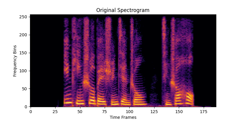
将音频文件重采样为 16000Hz,选取 3 秒的数据,转换为频谱,然后通过两层 Conv2D 进行处理,并可视化原始频谱和每层 Conv2D 的特征图。
python
import torch
import torch.nn as nn
import matplotlib.pyplot as plt
import librosa
import numpy as np
# 定义 Conv2D 模型
class Conv2DModel(nn.Module):
def __init__(self):
super(Conv2DModel, self).__init__()
self.conv1 = nn.Conv2d(in_channels=1, out_channels=2, kernel_size=(3, 3), stride=1, padding=1)
self.conv2 = nn.Conv2d(in_channels=2, out_channels=2, kernel_size=(5, 5), stride=1, padding=2)
def forward(self, x):
x = self.conv1(x)
x = self.conv2(x)
return x
# 1. 读取音频文件并处理
file_path = 'test.wav'
waveform, sample_rate = librosa.load(file_path, sr=16000, mono=True)
# 选取 3 秒的数据
start_sample = int(1.5 * sample_rate)
end_sample = int(4.5 * sample_rate)
audio_segment = waveform[start_sample:end_sample]
# 2. 转换为频谱
n_fft = 512
hop_length = 256
spectrogram = librosa.stft(audio_segment, n_fft=n_fft, hop_length=hop_length)
spectrogram_db = librosa.amplitude_to_db(np.abs(spectrogram))
# 将频谱转换为 PyTorch 张量并调整形状
spectrogram_tensor = torch.tensor(spectrogram_db, dtype=torch.float32).unsqueeze(0).unsqueeze(
0) # (1, 1, height, width)
# 打印原始频谱的维度
print(f"Original spectrogram shape: {spectrogram_tensor.shape}")
# 3. 创建模型实例
model = Conv2DModel()
# 打印每一层卷积层的权重形状
print(f"Conv2D Layer 1 weights shape: {model.conv1.weight.shape}")
print(f"Conv2D Layer 1 bias shape: {model.conv1.bias.shape}")
print(f"Conv2D Layer 2 weights shape: {model.conv2.weight.shape}")
print(f"Conv2D Layer 2 bias shape: {model.conv2.bias.shape}")
# 进行前向传播以获取每一层的输出
output1 = model.conv1(spectrogram_tensor) # 第一层输出
output2 = model.conv2(output1) # 第二层输出
# 打印每一层的输出形状
print(f"Output shape after Conv2D Layer 1: {output1.shape}")
print(f"Output shape after Conv2D Layer 2: {output2.shape}")
# 4. 可视化原始频谱
plt.figure(figsize=(8, 4))
plt.imshow(spectrogram_db, aspect='auto', origin='lower', cmap='inferno')
plt.title("Original Spectrogram")
plt.xlabel("Time Frames")
plt.ylabel("Frequency Bins")
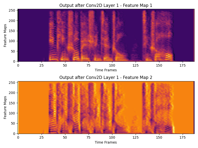
# 可视化第一层输出的所有特征图
plt.figure(figsize=(8, 6))
for i in range(output1.shape[1]): # 遍历每个特征图
plt.subplot(output1.shape[1], 1, i + 1) # 只绘制特征图
plt.imshow(output1[0, i, :, :].detach().numpy(), aspect='auto', origin='lower', cmap='inferno')
plt.title(f"Output after Conv2D Layer 1 - Feature Map {i + 1}")
plt.xlabel("Time Frames")
plt.ylabel("Feature Maps")
plt.tight_layout()
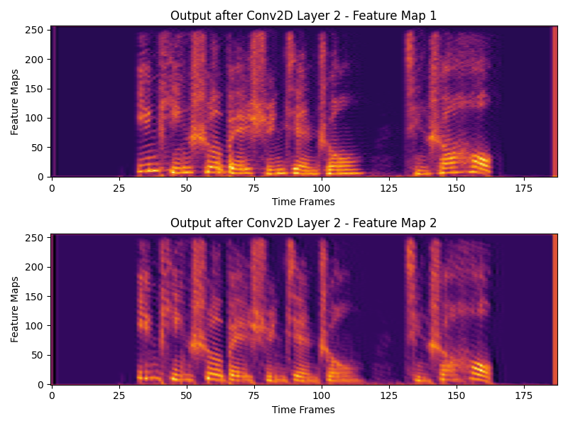
# 6. 可视化第二层输出的特征图
plt.figure(figsize=(8, 6))
for i in range(output2.shape[1]): # 遍历每个特征图
plt.subplot(output2.shape[1], 1, i + 1) # 5个子图
plt.imshow(output2[0, i, :, :].detach().numpy(), aspect='auto', origin='lower', cmap='inferno')
plt.title(f"Output after Conv2D Layer 2 - Feature Map {i + 1}")
plt.xlabel("Time Frames")
plt.ylabel("Feature Maps")
plt.tight_layout()
plt.show()
python
Original spectrogram shape: torch.Size([1, 1, 257, 188])
Conv2D Layer 1 weights shape: torch.Size([2, 1, 3, 3])
Conv2D Layer 1 bias shape: torch.Size([2])
Conv2D Layer 2 weights shape: torch.Size([2, 2, 5, 5])
Conv2D Layer 2 bias shape: torch.Size([2])
Output shape after Conv2D Layer 1: torch.Size([1, 2, 257, 188])
Output shape after Conv2D Layer 2: torch.Size([1, 2, 257, 188])