背景
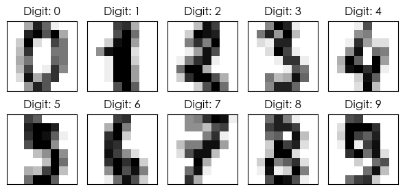
digits 手写数字数据集,1797个样本,8x8像素灰度图像(64个特征),10个类别(0-9)
作为多分类任务的玩具数据,需要使用分类方法进行分析
步骤
- 加载数据集
- 拆分训练集、测试集
- 数据预处理(标准化)
- 选择模型
- 模型训练(拟合)
- 测试模型效果
- 评估模型
分析方法
对数据集使用 7 种分类方法进行分析
- K 近邻(K-NN)
- 决策树
- 支持向量机(SVM)
- 逻辑回归
- 随机森林
- 朴素贝叶斯
- 多层感知机(MLP)
代码
python
from sklearn.datasets import load_digits

from sklearn.model_selection import train_test_split
from sklearn.preprocessing import StandardScaler
from sklearn.decomposition import PCA

from sklearn.neighbors import KNeighborsClassifier
from sklearn.tree import DecisionTreeClassifier
from sklearn.svm import SVC
from sklearn.linear_model import LogisticRegression
from sklearn.ensemble import RandomForestClassifier
from sklearn.naive_bayes import GaussianNB
from sklearn.neural_network import MLPClassifier

from sklearn.metrics import accuracy_score, classification_report, roc_curve, auc
from sklearn.preprocessing import label_binarize

import matplotlib.pyplot as plt
import numpy as np

# 设置 Matplotlib 字体以正确显示中文
# 尝试使用多种常见中文字体,提高跨平台兼容性
plt.rcParams['font.sans-serif'] = ['SimHei', 'WenQuanYi Zen Hei', 'STHeiti', 'Arial Unicode MS']
# 解决保存图像时负号'-'显示为方块的问题
plt.rcParams['axes.unicode_minus'] = False

def perform_digits_analysis():
    """
    使用 scikit-learn 对手写数字数据集进行全面的分析。
    该函数包含数据加载、预处理、模型训练、评估和 ROC/AUC 可视化。
    """
    print("--- 正在加载手写数字数据集 ---")
    # 加载手写数字数据集
    digits = load_digits()

    # 获取数据特征和目标标签
    X = digits.data
    y = digits.target
    target_names = [str(i) for i in digits.target_names]

    print("\n--- 数据集概览 ---")
    print(f"数据形状: {X.shape}")
    print(f"目标名称: {target_names}")

    # 将数据集划分为训练集和测试集
    X_train, X_test, y_train, y_test = train_test_split(X, y, test_size=0.3, random_state=42)

    print("\n--- 数据划分结果 ---")
    print(f"训练集形状: {X_train.shape}")
    print(f"测试集形状: {X_test.shape}")

    # 数据标准化
    print("\n--- 正在对数据进行标准化处理 ---")
    scaler = StandardScaler()
    X_train_scaled = scaler.fit_transform(X_train)
    X_test_scaled = scaler.transform(X_test)

    # 定义并训练多个分类器模型
    models = {
        "K近邻 (K-NN)": KNeighborsClassifier(n_neighbors=3),
        "决策树": DecisionTreeClassifier(random_state=42),
        "支持向量机 (SVM)": SVC(kernel='rbf', C=1.0, random_state=42, probability=True), # 必须设置 probability=True 来获取概率
        "逻辑回归": LogisticRegression(random_state=42, max_iter=1000),
        "随机森林": RandomForestClassifier(random_state=42),
        "朴素贝叶斯": GaussianNB(),
        "多层感知器 (MLP)": MLPClassifier(random_state=42, max_iter=300)
    }

    print("\n--- 模型训练与评估 ---")
    for name, model in models.items():
        print(f"\n--- 正在训练 {name} 模型 ---")
        # 使用标准化后的训练数据对模型进行拟合 (训练)
        model.fit(X_train_scaled, y_train)

        # 在标准化后的测试集上进行预测
        y_pred = model.predict(X_test_scaled)

        # 评估模型性能
        accuracy = accuracy_score(y_test, y_pred)
        report = classification_report(y_test, y_pred, target_names=target_names)

        print(f"{name} 模型的准确率: {accuracy:.4f}")
        print(f"{name} 模型的分类报告:\n{report}")

    print("\n--- ROC 曲线和 AUC 对比 ---")
    # 创建一个包含多个子图的图表
    num_models = len(models)
    cols = 3
    rows = (num_models + cols - 1) // cols
    fig, axes = plt.subplots(rows, cols, figsize=(18, 6 * rows))
    axes = axes.flatten()

    # 将多分类标签二值化,用于 ROC 曲线计算
    y_test_bin = label_binarize(y_test, classes=np.arange(10))

    # 循环遍历每个模型并绘制 ROC 曲线
    for i, (name, model) in enumerate(models.items()):
        ax = axes[i]

        # 获取每个类别的预测概率
        if hasattr(model, "predict_proba"):
            y_score = model.predict_proba(X_test_scaled)
        else: # 对于 SVC 这种没有 predict_proba 的模型,使用 decision_function
            y_score = model.decision_function(X_test_scaled)

        # 计算每个类别的 ROC 曲线和 AUC
        fpr = dict()
        tpr = dict()
        roc_auc = dict()
        for j in range(len(target_names)):
            fpr[j], tpr[j], _ = roc_curve(y_test_bin[:, j], y_score[:, j])
            roc_auc[j] = auc(fpr[j], tpr[j])

        # 计算微平均 ROC 曲线和 AUC
        fpr["micro"], tpr["micro"], _ = roc_curve(y_test_bin.ravel(), y_score.ravel())
        roc_auc["micro"] = auc(fpr["micro"], tpr["micro"])

        # 绘制所有类别的 ROC 曲线并填充
        for j in range(len(target_names)):
            ax.plot(fpr[j], tpr[j], label=f'类别 {j} (AUC = {roc_auc[j]:.2f})', alpha=0.7)
            ax.fill_between(fpr[j], tpr[j], alpha=0.1)

        # 绘制微平均 ROC 曲线
        ax.plot(fpr["micro"], tpr["micro"], label=f'微平均 (AUC = {roc_auc["micro"]:.2f})',
                color='deeppink', linestyle=':', linewidth=4)

        # 绘制对角线 (随机猜测)
        ax.plot([0, 1], [0, 1], 'k--', lw=2)

        # 设置图表属性
        ax.set_xlim([0.0, 1.0])
        ax.set_ylim([0.0, 1.05])
        ax.set_xlabel('假正率 (FPR)')
        ax.set_ylabel('真正率 (TPR)')
        ax.set_title(f'{name} - ROC 曲线')
        ax.legend(loc="lower right", fontsize='small')
        ax.grid(True)

    # 隐藏未使用的子图边框
    for j in range(num_models, len(axes)):
        axes[j].axis('off')

    plt.tight_layout()
    plt.show()

# 确保代码在作为主程序运行时才执行
if __name__ == "__main__":
    perform_digits_analysis()
结果
不同模型的 ROC 及 AUC 的对比
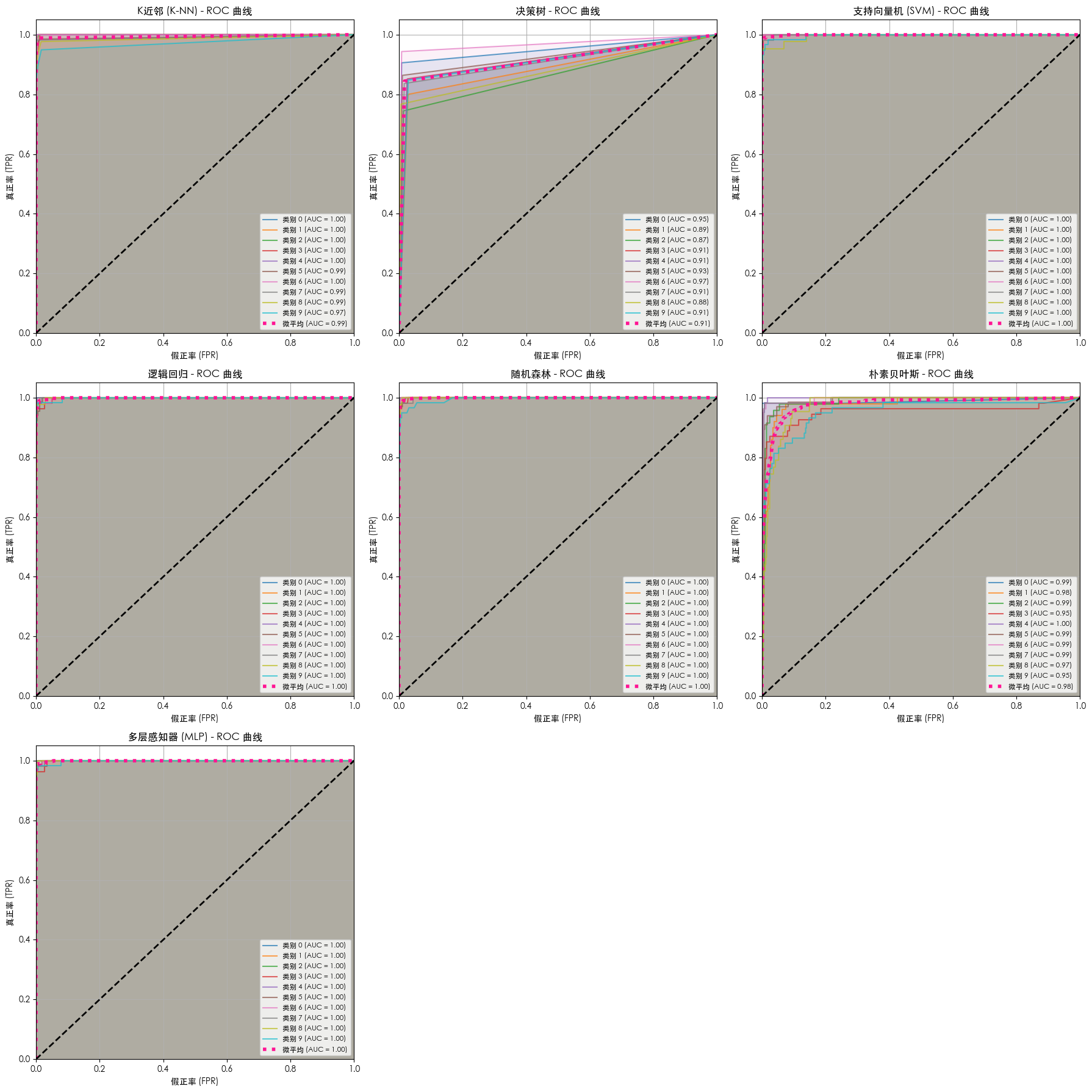
详情
--- 正在训练 K近邻 (K-NN) 模型 ---
K近邻 (K-NN) 模型的准确率: 0.9685
K近邻 (K-NN) 模型的分类报告:
              precision    recall  f1-score   support

           0       1.00      1.00      1.00        53
           1       0.94      1.00      0.97        50
           2       0.96      0.98      0.97        47
           3       0.94      0.94      0.94        54
           4       0.98      0.98      0.98        60
           5       0.98      0.97      0.98        66
           6       0.96      1.00      0.98        53
           7       1.00      0.98      0.99        55
           8       0.95      0.93      0.94        43
           9       0.95      0.90      0.92        59

    accuracy                           0.97       540
   macro avg       0.97      0.97      0.97       540
weighted avg       0.97      0.97      0.97       540


--- 正在训练 决策树 模型 ---
决策树 模型的准确率: 0.8444
决策树 模型的分类报告:
              precision    recall  f1-score   support

           0       0.92      0.91      0.91        53
           1       0.74      0.80      0.77        50
           2       0.83      0.74      0.79        47
           3       0.78      0.85      0.81        54
           4       0.81      0.85      0.83        60
           5       0.92      0.86      0.89        66
           6       0.93      0.94      0.93        53
           7       0.85      0.84      0.84        55
           8       0.92      0.77      0.84        43
           9       0.78      0.85      0.81        59

    accuracy                           0.84       540
   macro avg       0.85      0.84      0.84       540
weighted avg       0.85      0.84      0.84       540


--- 正在训练 支持向量机 (SVM) 模型 ---
支持向量机 (SVM) 模型的准确率: 0.9796
支持向量机 (SVM) 模型的分类报告:
              precision    recall  f1-score   support

           0       1.00      1.00      1.00        53
           1       1.00      1.00      1.00        50
           2       0.94      1.00      0.97        47
           3       0.98      0.94      0.96        54
           4       0.98      1.00      0.99        60
           5       0.97      1.00      0.99        66
           6       0.98      1.00      0.99        53
           7       1.00      0.96      0.98        55
           8       0.95      0.95      0.95        43
           9       0.98      0.93      0.96        59

    accuracy                           0.98       540
   macro avg       0.98      0.98      0.98       540
weighted avg       0.98      0.98      0.98       540


--- 正在训练 逻辑回归 模型 ---
逻辑回归 模型的准确率: 0.9704
逻辑回归 模型的分类报告:
              precision    recall  f1-score   support

           0       1.00      1.00      1.00        53
           1       0.98      0.94      0.96        50
           2       0.94      1.00      0.97        47
           3       1.00      0.93      0.96        54
           4       1.00      0.98      0.99        60
           5       0.95      0.95      0.95        66
           6       0.98      0.98      0.98        53
           7       1.00      0.98      0.99        55
           8       0.89      0.98      0.93        43
           9       0.95      0.97      0.96        59

    accuracy                           0.97       540
   macro avg       0.97      0.97      0.97       540
weighted avg       0.97      0.97      0.97       540


--- 正在训练 随机森林 模型 ---
随机森林 模型的准确率: 0.9741
随机森林 模型的分类报告:
              precision    recall  f1-score   support

           0       1.00      0.98      0.99        53
           1       0.96      0.98      0.97        50
           2       0.98      1.00      0.99        47
           3       0.98      0.96      0.97        54
           4       0.97      1.00      0.98        60
           5       0.97      0.95      0.96        66
           6       0.98      0.98      0.98        53
           7       0.98      0.98      0.98        55
           8       0.95      0.95      0.95        43
           9       0.97      0.95      0.96        59

    accuracy                           0.97       540
   macro avg       0.97      0.97      0.97       540
weighted avg       0.97      0.97      0.97       540


--- 正在训练 朴素贝叶斯 模型 ---
朴素贝叶斯 模型的准确率: 0.7833
朴素贝叶斯 模型的分类报告:
              precision    recall  f1-score   support

           0       0.96      0.98      0.97        53
           1       0.79      0.66      0.72        50
           2       0.86      0.40      0.55        47
           3       0.97      0.67      0.79        54
           4       1.00      0.58      0.74        60
           5       0.87      0.94      0.91        66
           6       0.83      0.98      0.90        53
           7       0.59      0.98      0.73        55
           8       0.51      0.88      0.65        43
           9       0.84      0.71      0.77        59

    accuracy                           0.78       540
   macro avg       0.82      0.78      0.77       540
weighted avg       0.83      0.78      0.78       540


--- 正在训练 多层感知器 (MLP) 模型 ---
多层感知器 (MLP) 模型的准确率: 0.9833
多层感知器 (MLP) 模型的分类报告:
              precision    recall  f1-score   support

           0       1.00      1.00      1.00        53
           1       1.00      1.00      1.00        50
           2       0.98      1.00      0.99        47
           3       1.00      0.94      0.97        54
           4       0.98      1.00      0.99        60
           5       0.97      0.98      0.98        66
           6       0.98      0.98      0.98        53
           7       1.00      0.98      0.99        55
           8       0.93      0.98      0.95        43
           9       0.98      0.97      0.97        59

    accuracy                           0.98       540
   macro avg       0.98      0.98      0.98       540
weighted avg       0.98      0.98      0.98       540