逻辑回归实践

目录

一、数据获取

二、数据处理与数据集制作

三、逻辑回归

---

一、数据获取

通过爬虫获取图片数据。

import requests
import re
import os
import time
headers = {'User-Agent':'Mozilla/5.0 (Windows NT 10.0; Win64; x64) AppleWebKit/537.36 (KHTML, like Gecko) Chrome/84.0.4147.125 Safari/537.36'}
name = input('您要爬取什么图片')
num = 0
num_1 = 0
num_2 = 0
x = input('您要爬取几张呢?，输入1等于60张图片。')
list_1 = []
for i in range(int(x)):
    name_1 = os.getcwd()
    name_2 = os.path.join(name_1,'图片')
    url = 'https://image.baidu.com/search/flip?tn=baiduimage&ie=utf-8&word='+name+'&pn='+str(i*30)
    res = requests.get(url,headers=headers)
    htlm_1 = res.content.decode()
    a = re.findall('"objURL":"(.*?)",',htlm_1)
    if not os.path.exists(name_2):
        os.makedirs(name_2)
    for b in a:
        try:
            b_1 = re.findall('https:(.*?)&',b)
            b_2 = ''.join(b_1)
            if b_2 not in list_1:
                num = num +1
                img = requests.get(b)
                f = open(os.path.join(name_1,'图片',name+str(num)+'.png'),'ab')
                print('---------正在下载第'+str(num)+'张图片----------')
                f.write(img.content)
                f.close()
                list_1.append(b_2)
            elif b_2 in list_1:
                num_1 = num_1 + 1 
                continue
        except Exception as e:
            print('---------第'+str(num)+'张图片无法下载----------')
            num_2 = num_2 +1
            continue
print('下载完成,总共下载{}张,成功下载:{}张,重复下载:{}张,下载失败:{}张'.format(num+num_1+num_2,num,num_1,num_2))
​

结果：

二、数据处理与数据集制作

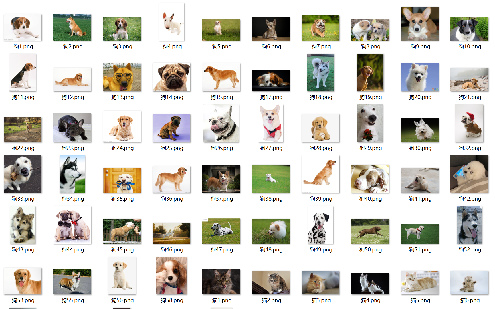
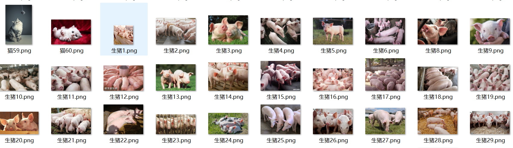
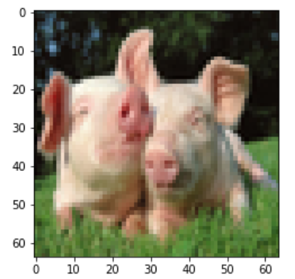
本次学习，通过逻辑回归识别猪的图片。通过网络爬虫分别爬取猪，猫，狗的图片，来做是否是猪的预测。

（1）数据处理：

1. 手动筛除一些图片

2. 图片标准化 长度宽度为64*64

（2）标准化代码

from PIL import Image
import os
## 说明：输入原始图像路径和新建图像文件夹名称 默认修改出长度宽度为64*64
def stdimage(pathorg,name,pathnew=None,width=64,length=64):
    #检查文件是否建立
    if pathnew == None: # 如果没有手动创建
        tage = os.path.exists(os.getcwd()+'\\'+name) #检查一下是否属实
        if not tage: #没有整个新文件夹
            os.mkdir(os.getcwd()+"\\"+name) #创建文件夹，name
        image_path = os.getcwd()+"\\"+name+"\\"
    else:#已经手动创建
        tage = os.path.exists(pathnew+"\\"+name)
        if not tage:
            path = os.getcwd()
            os.mkdir(path+"\\"+name)
        image_path = path +"\\"+name+"\\"
        
    ## 开始处理
    i = 1# 从一开始 
    list_name = os.listdir(pathorg) #获取图片名称列表
    for item in list_name:
        #检查是否有图片
        tage = os.path.exists(pathorg+str(i)+'.png')
        if not tage:
            image = Image.open(pathorg+'\\'+item)
            std = image.resize((width,length),Image.ANTIALIAS)
            ## 模式为RGB
            if not std.mode == "RGB":
                std = std.convert('RGB')
            std.save(image_path+str(i)+'.png')
        i+=1

（3）数据集制作

将图片数据制作成pyh5数据来保存，方便使用和共享。

首先将标准化好的图片变为numpy数组。

import numpy as np
import matplotlib.pyplot as plt
import h5py
import os
​
# 创建图片的numpy数组。
# 输入图片的path然后for循环建立rgb图片数组。
def creatdata(path):
    im_name_list = os.listdir(path)
    all_data =[]
    for item in im_name_list:
        try:
            all_data.append(plt.imread(path+'\\'+item).tolist())
        except:
            print(item+" open error ")
    return all_data
data = creatdata(r"F:\JupyterLab\CNN\stdimage")

再将data数据保存到pyh5文件中

import h5py
import numpy as np
​
# 准备数据
a = np.zeros((112, 1))  # 假设这是训练集的标签为0的数据
b = np.ones((166, 1))   # 假设这是训练集的标签为1的数据
c = np.vstack((a, b))   # 合并标签数据
​
# 假设 data 是训练集的特征数据
# data = ...  # 你需要定义 data，例如 data = np.random.rand(278, 64, 64, 3)
​
# 类别名称
d = np.array([['nopig'], ['pig']], dtype=h5py.string_dtype())
​
# 写入 HDF5 文件
with h5py.File("train_pig.h5", "w") as f:
    f.create_dataset("train_set_x", data=data)  # 确保 data 已定义
    f.create_dataset("train_set_y", data=c)
    f.create_dataset("classes_list", data=d)

三、逻辑回归

（1）加载数据

将我们制作好的数据取出来，并且可视化。

import matplotlib.pyplot as plt
import h5py
import numpy as np
train_data = h5py.File("train_pig.h5","r")
train_set_x_orig = np.array(train_data['train_set_x'][:])
train_set_y_orig = np.array(train_data['train_set_y'][:])
classes = np.array(train_data["classes_lsit"][:])
train_set_y_orig=train_set_y_orig.reshape((1,train_set_y_orig.shape[0]))
def plot_data(a):
    plt.imshow(train_set_x_orig[a])
plot_data(1)
plot_data(118)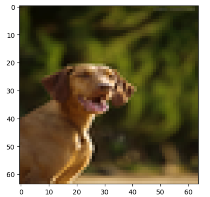

（2）训练集

train_set_x_f = train_set_x_orig.reshape(train_set_x_orig.shape[0],-1).T

（3）逻辑回归

准备好搭建的基本函数和方法

def sigmod(z):
    s= 1/(1+np.exp(-z))
    return s
def cast_TD(w,b,X,Y):
    """
    实现前向和后向传播的成本函数及其梯度。
    参数：
        w  - 权重，大小不等的数组（num_px * num_px * 3，1）
        b  - 偏差，一个标量
        X  - 矩阵类型为（num_px * num_px * 3，训练数量）
        Y  - 真正的“标签”矢量（如果非猫则为0，如果是猫则为1），矩阵维度为(1,训练数据数量)
​
    返回：
        cost- 逻辑回归的负对数似然成本
        dw  - 相对于w的损失梯度，因此与w相同的形状
        db  - 相对于b的损失梯度，因此与b的形状相同
    """
    m = X.shape[1]
    
    ##正向传播
    ## j的定义式
    A = sigmod(np.dot(w.T,X)+b)
    cost = (-1/m)*np.sum(Y * np.log(A)+(1-Y)*(np.log(1-A)))
    
    ## 反向传播
    ## 计算dw，db
    dw = (1/m)*np.dot(X,(A-Y).T)
    db = (1/m)*np.sum(A-Y)
    
    assert(dw.shape == w.shape)
    assert(db.dtype == float)
    cost = np.squeeze(cost)
    assert(cost.shape == ())
    
    grade = {
        "dw" : dw,
        "db" : db
    }
    
    return (grade , cost)
def changew(w , b , X , Y , times , alpha , print_cost = False):
    """
    此函数通过运行梯度下降算法来优化w和b
    
    参数：
        w  - 权重，大小不等的数组（num_px * num_px * 3，1）
        b  - 偏差，一个标量
        X  - 维度为（num_px * num_px * 3，训练数据的数量）的数组。
        Y  - 真正的“标签”矢量（如果非猫则为0，如果是猫则为1），矩阵维度为(1,训练数据的数量)
        times  - 优化循环的迭代次数
        alpha  - 梯度下降更新规则的学习率
        print_cost  - 每100步打印一次损失值
    
    返回：
        params  - 包含权重w和偏差b的字典
        grads  - 包含权重和偏差相对于成本函数的梯度的字典
        成本 - 优化期间计算的所有成本列表，将用于绘制学习曲线。
    
    提示：
    我们需要写下两个步骤并遍历它们：
        1）计算当前参数的成本和梯度，使用propagate（）。
        2）使用w和b的梯度下降法则更新参数。
    """
    costs = []
    ## 开始迭代
    for i in range(times):
        grads,cost =cast_TD(w,b,X,Y)
        dw = grads["dw"]
        db = grads["db"]
        w= w - alpha*dw
        b = b - alpha*db
        
        if i % 100 == 0:
            costs.append(cost)
            
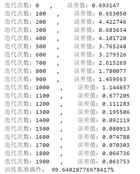
        if(print_cost) and (i%100==0):
            print("迭代次数：%i   ,    误差值：%f" % (i,cost))
            
    p = {
        "w":w,
        "b":b
    }
    
    grads = {
        "dw":dw,
        "db":db
    }
    
    return (p,grads,costs)
def initnet(a):
    w = np.zeros(shape = (a,1))
    b= 0 
    assert(w.shape == (a,1))
    assert(isinstance(b,float) or isinstance(b,int))
    return (w,b)
def yuce(w,b,X):
    """
    使用学习逻辑回归参数logistic （w，b）预测标签是0还是1，
    
    参数：
        w  - 权重，大小不等的数组（num_px * num_px * 3，1）
        b  - 偏差，一个标量
        X  - 维度为（num_px * num_px * 3，训练数据的数量）的数据
    
    返回：
        Y_prediction  - 包含X中所有图片的所有预测【0 | 1】的一个numpy数组（向量）
    
    """
    m = X.shape[1]
    Yyuce = np.zeros((1,m)) #设置一个矩阵来存放预测值
    w = w.reshape(X.shape[0],1)
    
    A = sigmod(np.dot(w.T,X)+b)
    for i in range(A.shape[1]):
        Yyuce[0,i] = 1 if A[0,i]> 0.5 else 0
        
    assert(Yyuce.shape == (1,m))
    
    return Yyuce
def logitic(X_train,Y_train,times=2000,alpha = 0.1,print_cost = False):
    """
    通过调用之前实现的函数来构建逻辑回归模型
    
    参数：
        X_train  - numpy的数组,维度为（num_px * num_px * 3，m_train）的训练集
        Y_train  - numpy的数组,维度为（1，m_train）（矢量）的训练标签集
        X_test   - numpy的数组,维度为（num_px * num_px * 3，m_test）的测试集
        Y_test   - numpy的数组,维度为（1，m_test）的（向量）的测试标签集
        times  - 表示用于优化参数的迭代次数的超参数
        alpha  - 表示logitic（）更新规则中使用的学习速率的超参数
        print_cost  - 设置为true以每100次迭代打印成本
    
    返回：
        res  - 包含有关模型信息的字典。
    """
    w , b = initnet(X_train.shape[0])
    
    p,grads,costs = changew(w,b,X_train,Y_train,times,alpha,print_cost)
    
    w , b = p["w"],p["b"]
    
#   预测，检查模型的可靠性
    Yyuce_train = yuce(w,b,X_train)
    
#     打印准确性
    print("训练集准确性：",format(100 - np.mean(np.abs(Y_train-Yyuce_train))*100)+"%")
    
    
    d = {
        "costs":costs, # 作图时候可以使用代价，看代价的变化
        "Yyuce_train":Yyuce_train,
        "w":w,
        "b":b,
        "alpha":alpha,
        "times":times
    }
    
    return d

开始使用

d = logitic(train_set_x_f,train_set_y_orig,times = 2000,alpha = 0.01,print_cost=True)
costs = np.squeeze(d['costs'])
plt.plot(costs)
plt.ylabel('cost')
plt.xlabel('times')
plt.title("Alpha = "+ str(d["alpha"]))
plt.show()

结果