Deep Learning|03 Overview of Machine Learning

Deep Learning|03 Overview of Machine Learning

In layman's terms, machine learning (ML) is the process of enabling computers to automatically learn and acquire certain knowledge from numerous and massive data. In the early period of engineering, ML was always called pattern recognition, which tended to solve certain application tasks that are easy for humans.

Fundamental concepts

There are some basic concepts needed to learn:

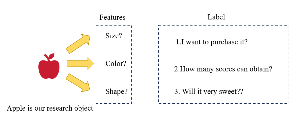
• Feature : Attribute. Generally, we use x∈Rn\boldsymbol{x} \in \mathbb{R}^nx∈Rn to represent the features of an object.

• Label : Generally, we use y∈Ry \in \mathbb{R}y∈R to represent the label of an object.

• Sample: Instance.

• Data Set: Includes training set and test set.

Suppose the training set D\mathcal{D}D consists of NNN samples, where each sample is Identically and Independently Distributed (IID)---that is, they are independently drawn from the same data distribution. It is denoted as:
D={(x(1),y(1)),(x(2),y(2)),...,(x(N),y(N))}. \mathcal{D} = \{(\boldsymbol{x}^{(1)}, y^{(1)}), (\boldsymbol{x}^{(2)}, y^{(2)}), \dots, (\boldsymbol{x}^{(N)}, y^{(N)})\}. D={(x(1),y(1)),(x(2),y(2)),...,(x(N),y(N))}.

Given the training set D\mathcal{D}D, we hope the computer can automatically find an "optimal" function f∗(x)f^*(\boldsymbol{x})f∗(x) from a function set F={f1(x),f2(x),... }\mathcal{F} = \{f_1(\boldsymbol{x}), f_2(\boldsymbol{x}), \dots\}F={f1(x),f2(x),...} to approximate the true mapping relationship between the feature vector x\boldsymbol{x}x and the label yyy of each sample. For a sample x\boldsymbol{x}x, we can use the function f∗(x)f^*(\boldsymbol{x})f∗(x) to predict the value of its label as:
y^=f∗(x) \hat{y} = f^*(\boldsymbol{x}) y^=f∗(x)

or predict the conditional probability of the label as:
p^(y∣x)=fy∗(x) \hat{p}(y \mid \boldsymbol{x}) = f_y^*(\boldsymbol{x}) p^(y∣x)=fy∗(x)

How to find this "optimal" function f∗(x)f^*(\boldsymbol{x})f∗(x) is the key to machine learning, which is generally accomplished through a learning algorithm A\mathcal{A}A. This search process is usually called the learning or training process.

In this way, the next time we buy mangoes from the market (test samples), we can predict the quality of the mangoes using the learned function f∗(x)f^*(\boldsymbol{x})f∗(x) based on the features of the mangoes. For the fairness of evaluation, we still draw a set of mangoes as the test set D′\mathcal{D}'D′ identically and independently, and test all mangoes in the test set to calculate the accuracy of the prediction results:
Acc(f∗(x))=1∣D′∣∑I(f∗(x)=y) \text{Acc}(f^*(\boldsymbol{x})) = \frac{1}{|\mathcal{D}'|} \sum \mathrm{I}\left(f^*(\boldsymbol{x}) = y\right) Acc(f∗(x))=∣D′∣1∑I(f∗(x)=y)

where I(⋅)\mathrm{I}(\cdot)I(⋅) is the indicator function, and ∣D′∣|\mathcal{D}'|∣D′∣ is the size of the test set.

Three fundamental elements of ML

For an ML task, the input space X\mathcal{X}X and output space Y\mathcal{Y}Y form a sample space and generate a data set: (x,y)∈X×Y(\boldsymbol{x}, y) \in \mathcal{X} \times \mathcal{Y}(x,y)∈X×Y. The goal of ML is to find a model to approximate the mapping from x\boldsymbol{x}x to yyy, including functional mapping and conditional probability distribution.

Since we do not know the real mapping, we assume a function set F\mathcal{F}F (called the Hypothesis Space) and find the best element f∗∈Ff^* \in \mathcal{F}f∗∈F to replace the real mapping. Generally, the hypothesis space F\mathcal{F}F is a parameterized function family:
F={f(x;θ)∣θ∈Rm} \mathcal{F} = \{f(\boldsymbol{x}; \boldsymbol{\theta}) \mid \boldsymbol{\theta} \in \mathbb{R}^m\} F={f(x;θ)∣θ∈Rm}

where f(x;θ)f(\boldsymbol{x}; \boldsymbol{\theta})f(x;θ) is a function with θ\boldsymbol{\theta}θ as the parameter, and mmm is the number of parameters.

Common hypothesis spaces can be divided into linear and nonlinear types, corresponding to linear models and nonlinear models.

Linear Model

The hypothesis space of a linear model is a parameterized family of linear functions, i.e.:
f(x;θ)=w⊤x+b f(\boldsymbol{x}; \boldsymbol{\theta}) = \boldsymbol{w}^\top \boldsymbol{x} + b f(x;θ)=w⊤x+b

where the parameter θ\boldsymbol{\theta}θ includes the weight vector w\boldsymbol{w}w and the bias bbb.

Nonlinear Model

A generalized nonlinear model can be written as a linear combination of multiple nonlinear basis functions ϕ(x)\phi(\boldsymbol{x})ϕ(x):
f(x;θ)=w⊤ϕ(x)+b. f(\boldsymbol{x}; \boldsymbol{\theta}) = \boldsymbol{w}^\top \phi(\boldsymbol{x}) + b. f(x;θ)=w⊤ϕ(x)+b.

where ϕ(x)=[ϕ1(x),ϕ2(x),...,ϕK(x)]⊤\phi(\boldsymbol{x}) = [\phi_1(\boldsymbol{x}), \phi_2(\boldsymbol{x}), \dots, \phi_K(\boldsymbol{x})]^\topϕ(x)=[ϕ1(x),ϕ2(x),...,ϕK(x)]⊤ is a vector composed of KKK nonlinear basis functions, and the parameter θ\boldsymbol{\theta}θ includes the weight vector w\boldsymbol{w}w and the bias bbb.

If ϕ(x)\phi(\boldsymbol{x})ϕ(x) itself is a learnable basis function (e.g.):
ϕk(x)=h(wk⊤ϕ′(x)+bk),∀1≤k≤K \phi_k(\boldsymbol{x}) = h\left( \boldsymbol{w}_k^\top \phi'(\boldsymbol{x}) + b_k \right), \quad \forall 1 \leq k \leq K ϕk(x)=h(wk⊤ϕ′(x)+bk),∀1≤k≤K

where h(⋅)h(\cdot)h(⋅) is a nonlinear function, ϕ′(x)\phi'(\boldsymbol{x})ϕ′(x) is another set of basis functions, and wk\boldsymbol{w}_kwk and bkb_kbk are learnable parameters, then f(x;θ)f(\boldsymbol{x}; \boldsymbol{\theta})f(x;θ) is equivalent to a neural network model.

Learning Principle

A good model f(x;θ∗)f(\boldsymbol{x}; \boldsymbol{\theta}^*)f(x;θ∗) should be as consistent as possible with the true mapping values on D={(xn,yn)}n=1N\mathcal{D} = \left\{(\boldsymbol{x}n, y_n)\right\}{n=1}^ND={(xn,yn)}n=1N, i.e.:
∣f(x;θ∗)−y∣<ε,∀(xn,yn)∈D \left|f(\boldsymbol{x}; \boldsymbol{\theta}^*) - y\right| < \varepsilon, \quad \forall (\boldsymbol{x}_n, y_n) \in \mathcal{D} ∣f(x;θ∗)−y∣<ε,∀(xn,yn)∈D

or consistent with the real conditional probability distribution pr(y∣x)p_r(y|\boldsymbol{x})pr(y∣x), i.e.:
∣fy(x;θ∗)−pr(y∣x)∣<ε,∀(xn,yn)∈D \left|f_y(\boldsymbol{x}; \boldsymbol{\theta}^*) - p_r(y|\boldsymbol{x})\right| < \varepsilon, \quad \forall (\boldsymbol{x}_n, y_n) \in \mathcal{D} ∣fy(x;θ∗)−pr(y∣x)∣<ε,∀(xn,yn)∈D

The quality of a model can be evaluated by the expected risk R(θ)\mathcal{R}(\boldsymbol{\theta})R(θ), defined as:
R(θ)=E(x,y)∼pr(x,y)[L(y,f(x;θ))] \mathcal{R}(\boldsymbol{\theta}) = \mathbb{E}_{(\boldsymbol{x}, y) \sim p_r(\boldsymbol{x}, y)} \left[\mathcal{L}(y, f(\boldsymbol{x}; \boldsymbol{\theta}))\right] R(θ)=E(x,y)∼pr(x,y)[L(y,f(x;θ))]

where pr(x,y)p_r(\boldsymbol{x}, y)pr(x,y) is the real distribution of the data, and L(y,f(x;θ))\mathcal{L}(y, f(\boldsymbol{x}; \boldsymbol{\theta}))L(y,f(x;θ)) (called the Loss Function) is used to measure the difference between the true label yyy and the predicted value f(x;θ)f(\boldsymbol{x}; \boldsymbol{\theta})f(x;θ).

Common loss functions are as follows:

1. 0-1 Loss Function
   L(y,f(x;θ))={0,y=f(x;θ)1,y≠f(x;θ) \mathcal{L}(y, f(\boldsymbol{x};\boldsymbol{\theta})) = \begin{cases} 0, & y = f(\boldsymbol{x};\boldsymbol{\theta}) \\ 1, & y \neq f(\boldsymbol{x};\boldsymbol{\theta}) \end{cases} L(y,f(x;θ))={0,1,y=f(x;θ)y=f(x;θ)

2. Quadratic Loss Function
   L(y,f(x;θ))=12[y−f(x;θ)]2 \mathcal{L}(y, f(\boldsymbol{x};\boldsymbol{\theta})) = \frac{1}{2}\left[y - f(\boldsymbol{x};\boldsymbol{\theta})\right]^2 L(y,f(x;θ))=21[y−f(x;θ)]2

3. Cross-Entropy Loss Function

   The cross-entropy loss function is generally used for classification problems. Assume the label y∈{1,⋯ ,C}y \in \{1, \cdots, C\}y∈{1,⋯,C} of a sample is a discrete category, and the output of the model f(x;θ)∈[0,1]Cf(\boldsymbol{x}; \theta) \in [0,1]^Cf(x;θ)∈[0,1]C is the conditional probability distribution of the category labels, i.e.:
   p(y=c∣x;θ)=fc(x;θ) p(y = c|\boldsymbol{x};\boldsymbol{\theta}) = f_c(\boldsymbol{x}; \boldsymbol{\theta}) p(y=c∣x;θ)=fc(x;θ)

   and it satisfies:
   fc(x;θ)∈[0,1],∑c=1Cfc(x;θ)=1. f_c(\boldsymbol{x}; \boldsymbol{\theta}) \in [0,1], \quad \sum_{c=1}^C f_c(\boldsymbol{x}; \boldsymbol{\theta}) = 1. fc(x;θ)∈[0,1],c=1∑Cfc(x;θ)=1.

We can use a CCC-dimensional one-hot vector y\boldsymbol{y}y to represent the sample label. Assume the label of a sample is kkk---then only the kkk-th dimension of the label vector y\boldsymbol{y}y is 1, and the other elements are 0. The label vector y\boldsymbol{y}y can be regarded as the true conditional probability distribution pr(y∣x)p_r(\boldsymbol{y}|\boldsymbol{x})pr(y∣x) of the sample label (i.e., the ccc-th dimension, denoted as ycy_cyc for 1≤c≤C1 \leq c \leq C1≤c≤C, is the true conditional probability of category ccc). If the category of a sample is kkk, the probability of it belonging to the kkk-th category is 1, and the probability of it belonging to other categories is 0.

For two probability distributions, cross-entropy is generally used to measure their difference. The cross-entropy between the true distribution y\boldsymbol{y}y of labels and the predicted distribution f(x;θ)f(\boldsymbol{x}; \theta)f(x;θ) of the model is:
L(y,f(x;θ))=−y⊺log⁡f(x;θ)=−∑c=1Cyclog⁡fc(x;θ) \mathcal{L}(\boldsymbol{y}, f(\boldsymbol{x}; \boldsymbol{\theta})) = -\boldsymbol{y}^\intercal \log f(\boldsymbol{x}; \boldsymbol{\theta}) = -\sum_{c=1}^C y_c \log f_c(\boldsymbol{x}; \boldsymbol{\theta}) L(y,f(x;θ))=−y⊺logf(x;θ)=−c=1∑Cyclogfc(x;θ)

For a one-hot label vector, the formula can be rewritten as:
L(y,f(x;θ))=−log⁡fy(x;θ) \mathcal{L}(\boldsymbol{y}, f(\boldsymbol{x}; \boldsymbol{\theta})) = -\log f_y(\boldsymbol{x}; \boldsymbol{\theta}) L(y,f(x;θ))=−logfy(x;θ)

It can be observed that the cross-entropy loss function is the negative log-likelihood.

4. Hinge Loss Function
   For a sample (x,y)(\boldsymbol{x}, y)(x,y) (where y∈{−1,1}y \in \{-1, 1\}y∈{−1,1} is the class label, and f(x)=w⊤x+bf(\boldsymbol{x}) = \boldsymbol{w}^\top \boldsymbol{x} + bf(x)=w⊤x+b is the model's output), the hinge loss is defined as:
   L(y,f(x))=max⁡(0,1−y⋅f(x)) \mathcal{L}(y, f(\boldsymbol{x})) = \max(0, 1 - y \cdot f(\boldsymbol{x})) L(y,f(x))=max(0,1−y⋅f(x))

The target of ML is to minimize the empirical risk on D\mathcal{D}D:
RDemp(θ)=∑n=1NL(y(n),f(x(n);θ))N \mathcal{R}^{\text{emp}}{\mathcal{D}}(\boldsymbol{\theta}) = \frac{\sum{n=1}^N \mathcal{L}(\boldsymbol{y}^{(n)}, f(\boldsymbol{x}^{(n)}; \boldsymbol{\theta}))}{N} RDemp(θ)=N∑n=1NL(y(n),f(x(n);θ))

Thus, the optimal parameter θ∗\boldsymbol{\theta}^*θ∗ can be calculated as:
θ∗=arg⁡min⁡θRDemp(θ) \boldsymbol{\theta}^* = \arg \min_{\boldsymbol{\theta}} \mathcal{R}^{\text{emp}}_{\mathcal{D}}(\boldsymbol{\theta}) θ∗=argθminRDemp(θ)

Optimization Algorithm

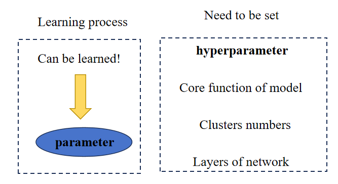
As shown in the figure:

Hyper-parameters need to be set manually, while parameters can be learned through certain optimization algorithms.

Gradient Descent

θt+1=θt−η⋅∇θRD(θ) \boldsymbol{\theta}{t+1} = \boldsymbol{\theta}{t} - \eta \cdot \nabla_{\boldsymbol{\theta}} \mathcal{R}_{\mathcal{D}}(\boldsymbol{\theta}) θt+1=θt−η⋅∇θRD(θ)

where η\etaη is the learning rate.

Based on the amount of data used in each iteration, Gradient Descent is mainly divided into three types:

• Batch Gradient Descent (BGD): Uses all training data to calculate the gradient in each iteration. Its advantage is stable gradients, while its disadvantage is low computational efficiency when the data volume is large.
• Stochastic Gradient Descent (SGD): Uses only a single training sample to calculate the gradient in each iteration. Its advantages are fast speed and the ability to avoid local optima, while its disadvantage is large gradient fluctuations.
• Mini-Batch Gradient Descent (MBGD): Uses a small batch of training samples (e.g., 32, 64, or 128 samples) to calculate the gradient in each iteration. It balances the stability of BGD and the efficiency of SGD, and is currently the most commonly used form in deep learning.

Linear Regression

From the perspective of ML, in linear regression, the independent variable x∈Rn\boldsymbol{x} \in \mathbb{R}^nx∈Rn is the feature vector of the sample, and the dependent variable is the label y∈Ry \in \mathbb{R}y∈R (a continuous value). The model is defined as:
f(x;w,b)=w⊤x+b f(\boldsymbol{x};\boldsymbol{w},b) = \boldsymbol{w}^\top \boldsymbol{x} + b f(x;w,b)=w⊤x+b

where w\boldsymbol{w}w and bbb are learnable parameters.

Define ⨁\bigoplus⨁ as the vector concatenation symbol. The linear regression equation can be rewritten as:
f(x^;w^)=w^⊤x^ f(\hat{\boldsymbol{x}};\hat{\boldsymbol{w}}) = \hat{\boldsymbol{w}}^\top \hat{\boldsymbol{x}} f(x^;w^)=w^⊤x^

where x^=x⨁1\hat{\boldsymbol{x}} = \boldsymbol{x} \bigoplus 1x^=x⨁1 and w^=w⨁b\hat{\boldsymbol{w}} = \boldsymbol{w} \bigoplus bw^=w⨁b.

It is easy to prove that the empirical risk function of linear regression is:
R(w^)=12∥y−X⊤w^∥ \mathcal{R}( \hat{\boldsymbol{w}} ) = \frac{1}{2}\|\boldsymbol{y} - X^\top \hat{\boldsymbol{w}}\| R(w^)=21∥y−X⊤w^∥

where XXX is ⨁Dx^\bigoplus_{\mathcal{D}} \hat{\boldsymbol{x}}⨁Dx^ (i.e., the matrix formed by concatenating all x^\hat{\boldsymbol{x}}x^ in the training set D\mathcal{D}D).

The optimal parameter w^∗\hat{\boldsymbol{w}}^*w^∗ is:
w^∗=(XX⊤)−1Xy \hat{\boldsymbol{w}}^* = (XX^\top)^{-1}X\boldsymbol{y} w^∗=(XX⊤)−1Xy

Bias-Variance Decomposition

The generalization error of a model can be decomposed into three parts: bias, variance, and irreducible noise:
ED[(y−f(x))2]⏟Generalization Error =(f∗(x)−ED[f(x)])2⏟Bias2+ED[(f(x)−ED[f(x)])2]⏟Variance+Var(ϵ)⏟Irreducible Noise \underbrace{\mathbb{E}\mathcal{D}\left[(y - f(\boldsymbol{x}))^2\right]}{\text{Generalization Error }} = \underbrace{(f^*(\boldsymbol{x}) - \mathbb{E}\mathcal{D}[f(\boldsymbol{x})])^2}{\text{Bias}^2} + \underbrace{\mathbb{E}\mathcal{D}\left[\left(f(\boldsymbol{x}) - \mathbb{E}\mathcal{D}[f(\boldsymbol{x})]\right)^2\right]}{\text{Variance}} + \underbrace{\text{Var}(\epsilon)}{\text{Irreducible Noise}} Generalization Error ED[(y−f(x))2]=Bias2 (f∗(x)−ED[f(x)])2+Variance ED[(f(x)−ED[f(x)])2]+Irreducible Noise Var(ϵ)

• Bias: Refers to the difference between the average performance of a model on different training sets and the optimal model. It measures the fitting ability of the model (a high bias indicates underfitting).
• Variance: Refers to the variation in model predictions across different training sets. It measures whether the model is prone to overfitting (a high variance indicates overfitting).
• Irreducible Noise: The inherent noise in the data, which cannot be eliminated by any model.

Feature Engineering

Different types of data have different spaces of raw features. This requires us to select or extract informative features as input for the computer.

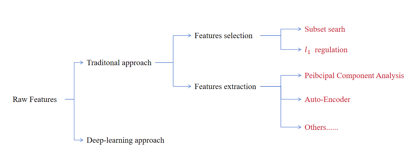
Feature Selection

Feature selection is a critical preprocessing step in machine learning and data mining. Its core goal is to select a subset of the most relevant features from the original feature set, while removing irrelevant, redundant, or noisy features. This process simplifies models, reduces computational costs, mitigates overfitting, and improves interpretability---all without significantly sacrificing predictive performance.

Feature Extraction

The core goal of feature extraction is to transform raw high-dimensional data into a lower-dimensional feature space by capturing the most informative patterns, while discarding noise, redundancy, or irrelevant details. Unlike feature selection (which selects a subset of original features), feature extraction creates new features that better represent the underlying structure of the data.