Transformer架构:手撸源码实践
1. 引言
Transformer架构自2017年在论文《Attention Is All You Need》中被提出以来,彻底改变了自然语言处理(NLP)领域。它摒弃了传统的循环神经网络(RNN)和卷积神经网络(CNN),完全基于注意力机制构建,成为现代大语言模型(如BERT、GPT系列)的基础架构。
本文将深入解析Transformer的核心组件,通过手写实现代码来帮助理解其内部工作机制。
2. Transformer整体架构
Transformer采用经典的编码器-解码器架构:
输入序列 → 编码器 → 解码器 → 输出序列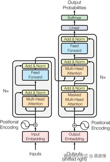
2.1 编码器(Encoder)
编码器由6个相同的层堆叠而成,每层包含两个子层:
- 多头自注意力机制(Multi-Head Self-Attention)
- 位置前馈网络(Position-wise Feed-Forward Networks)
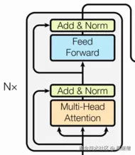 每层都使用残差连接和层归一化。
编码器可以表示为以下公式:
EncLayer(x)=LayerNorm(x+SelfAttention(x))
EncLayer(x)=LayerNorm(x+FFN(x))
完整的编码器层可以表示为:
EncoderLayer(x)=LayerNorm(LayerNorm(x+SelfAttention(x))+FFN(LayerNorm(x+SelfAttention(x))))
2.2 解码器(Decoder)
解码器也由6个相同的层堆叠而成,每层包含三个子层:
- 掩码多头自注意力机制(Masked Multi-Head Self-Attention)
- 编码器-解码器注意力机制(Encoder-Decoder Attention)
- 位置前馈网络(Position-wise Feed-Forward Networks)
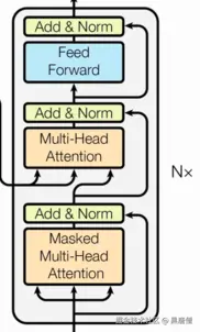 同样,每层都使用残差连接和层归一化。
解码器层可以表示为以下公式:
DecLayer(x,encout)=LayerNorm(x+MaskedSelfAttention(x))
DecLayer(x,encout)=LayerNorm(x+EncoderAttention(x,encout))
DecLayer(x,encout)=LayerNorm(x+FFN(x))
3. 核心组件详解
3.1 注意力机制(Attention)
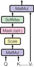
注意力机制是Transformer的核心,其数学表达式为:
Attention(Q,K,V)=softmax(dk QKT)V
其中:
- Q(Query):查询向量
- K(Key):键向量
- V(Value):值向量
- dk:键向量的维度
缩放因子 dk 1的作用是为了防止点积结果过大导致softmax函数梯度消失。
在我们的实现中,注意力机制的代码如下:
python
def attention(q, k, v, mask=None, dropout=None):
    """
    计算注意力机制

    Args:
        q: 查询矩阵 [batch_size, heads, seq_len, d_k]
        k: 键矩阵 [batch_size, heads, seq_len, d_k]
        v: 值矩阵 [batch_size, heads, seq_len, d_k]
        mask: 掩码矩阵,用于屏蔽某些位置
        dropout: dropout层

    Returns:
        tuple: (注意力输出, 注意力权重)
    """
    # 自注意力公式三步走

    # 第一步: q* k的转置除以根号d_k

    # 第二部: 判断是否做掩码, softmax层计算

    # 第三部: 乘以V
    # [batch_size, sqen_len, embed_dim]
    embed_dim = k.size(-1)
    # 计算Q和K的点积 [batch_size, heads, seq_len, seq_len]
    q_k = torch.matmul(q, k.transpose(-1,-2)) # batch_size, sqen_len, sqen_len
    # 缩放点积,除以根号d_k,防止梯度消失
    attn_weight = q_k / math.sqrt(embed_dim)

    if mask is not None:
        # 使用mask屏蔽不需要关注的位置,将被屏蔽位置的权重设为极小值
        attn_weight = attn_weight.masked_fill(mask == 0, -1e9)

    # 对注意力权重进行softmax归一化
    attn_weight = nn.functional.softmax(attn_weight, dim=-1)

    if dropout is not None:
        # 应用dropout防止过拟合
        attn_weight = dropout(attn_weight)

    # 使用注意力权重对V进行加权求和
    res = torch.matmul(attn_weight , v)

    return res, attn_weight
3.2 多头注意力(Multi-Head Attention)
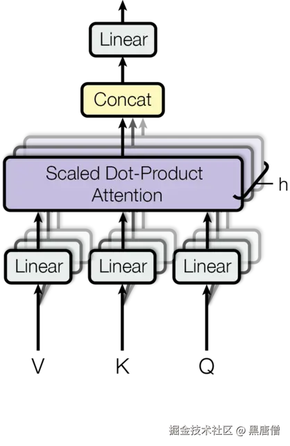
为了增强模型捕捉不同位置信息的能力,Transformer使用多头注意力机制:
MultiHead(Q,K,V)=Concat(head1,...,headh)WO
其中每个头计算为: headi=Attention(QWiQ,KWiK,VWiV)
多头注意力机制允许模型在不同表示子空间中并行关注信息,增强了模型的表达能力。
MultiHead计算的完整过程可以表示为:
MultiHead(Q,K,V)=Concat(head1,...,headh)WO
whereheadi=Attention(QWiQ,KWiK,VWiV)
多头注意力机制结构图
python
class MultiHeadAttention(nn.Module):
    """
    多头注意力机制
    将输入分割为多个头,分别计算注意力,然后合并结果
    """
    def __init__(self, heads, embed_dim, dropout_p=0.1):
        """
        初始化多头注意力

        Args:
            heads: 注意力头的数量
            embed_dim: 嵌入维度
            dropout_p: dropout概率
        """
        super().__init__()
        # 构建属性
        self.heads = heads
        self.embed_dim = embed_dim

        # 确保嵌入维度可以被头数整除
        assert embed_dim % heads  == 0
        # 计算每个头的维度
        self.d_k = embed_dim // heads
        # 构建4个线性层: 3个用于Q、K、V的线性变换,1个用于最终输出
        self.linears = clone_modules(nn.Linear(embed_dim, embed_dim), 4)
        # 实例化dropout
        self.dropout = nn.Dropout(dropout_p)

    def forward(self, q, k, v, mask=None):
        """
        前向传播

        Args:
            q: 查询 [batch_size, seq_len, embed_dim]
            k: 键 [batch_size, seq_len, embed_dim]
            v: 值 [batch_size, seq_len, embed_dim]
            mask: 掩码矩阵

        Returns:
            torch.Tensor: 多头注意力输出
        """
        if mask is not None:
            # 扩展mask的维度以匹配多头
            mask = mask.unsqueeze(0)
        batch_size = q.size(0)
        heads = self.heads
        embed_dim = q.size(-1)
        d_k = self.d_k
        # 拆分多头序列 + 做线性变换
        # 对Q、K、V分别应用线性变换,然后reshape为(batch_size, heads, seq_len, d_k)
        q, k, v = [linear(x)
                    .view(batch_size, -1, heads, d_k)
                    .transpose(1,2)
                    for linear,x in zip(self.linears,(q,k,v))]

        # 获取注意力机制输出
        output, attn_weight = attention(q, k, v, mask, self.dropout)
        # 合并多头到一个量中
        # 交换维度并合并heads和d_k维度
        res = output.transpose(1,2).contiguous().view(batch_size, -1, embed_dim)
        # 最后使用线性层做收尾处理
        return self.linears[-1](res)
3.3 位置编码(Positional Encoding)
由于自注意力机制本身不包含位置信息,Transformer引入位置编码来为模型提供序列中词的位置信息。
Transformer使用正弦和余弦函数生成位置编码:
PE(pos,2i)=sin(100002i/dmodelpos)
PE(pos,2i+1)=cos(100002i/dmodelpos)
其中:
- pos 是位置
- i 是维度
- dmodel 是模型维度
这种设计使得模型能够学习到相对位置信息,因为对于任意固定的偏移 k, PEpos+k 可以表示为 PEpos 的线性函数。
位置编码的完整公式可以表示为:
PE(pos,2i)=sin(100002i/dmodelpos)
PE(pos,2i+1)=cos(100002i/dmodelpos)
python
class PositionalEmbedding(nn.Module):
    """
    位置编码层
    为序列中每个位置生成独特的编码,使模型能够利用序列顺序信息
    """
    def __init__(self, max_length, embed_dim, dropout_p=0.1):
        """
        初始化位置编码层

        Args:
            max_length: 序列最大长度
            embed_dim: 嵌入维度
            dropout_p: dropout概率
        """
        super().__init__()
        self.max_length = max_length
        self.embed_dim = embed_dim

        # Dropout层用于防止过拟合
        self.dropout = nn.Dropout(p=dropout_p)

        # 创建位置编码矩阵 [max_length, embed_dim]
        pe = torch.zeros(max_length, embed_dim)   # [60, 512]

        # 生成位置信息 [max_length, 1]
        pos = torch.arange(0, max_length).unsqueeze(1) # [60, 1] = [[0],[1],[2], ...[59]]
        # 生成维度索引 0, 2, 4, ..., embed_dim-2 (只取偶数索引)
        tow_i = torch.arange(0, embed_dim, 2) # [256] = 0 2 4 6 8 .. 510  , 一共256个数
        # 计算角度频率参数
        tmp_v = torch.exp((math.log(10000) * -tow_i / self.embed_dim)) # [256]

        # 计算角度值:pos * 角度频率
        fn_v = tmp_v * pos # [256] * [60, 1]

        # 偶数位置使用sin编码
        pe[:, 0::2] = torch.sin(fn_v)
        # 奇数位置使用cos编码
        pe[:, 1::2] = torch.cos(fn_v)

        # 增加batch维度 [1, max_length, embed_dim]
        pe = pe.unsqueeze(0) # [1, 60, 512]

        # 注册为buffer,不会被更新,但会随模型保存和加载
        self.register_buffer('pe', pe)

    def forward(self, x): # 输入形状:[batch_size, seq_len, embed_dim]
        """
        前向传播

        Args:
            x: 输入张量 [batch_size, seq_len, embed_dim]

        Returns:
            torch.Tensor: 加入位置编码的张量 [batch_size, seq_len, embed_dim]
        """
        # 截取与输入序列长度相等的位置编码
        p_x = self.pe[:, :x.size(1)] # [1, seq_len, embed_dim]
        # 将位置编码与输入相加,并应用dropout
        res = self.dropout(p_x + x) # [batch_size, seq_len, embed_dim]

        return res
3.4 词嵌入与缩放(Embedding and Scaling)
Transformer中的Embedding层负责将离散的词汇转换为连续向量表示。为了保持数值稳定性,Transformer在词嵌入后进行缩放操作:
Embeddingscaled=Embedding×dmodel
词嵌入缩放的目的是平衡词嵌入和位置编码的数值范围,确保两者在数值上处于相近的量级,有助于模型训练的稳定性。
python
class Embeddings(nn.Module):
    """
    词嵌入层
    将词汇索引转换为密集向量表示
    """
    def __init__(self, input_size, embed_dim):
        """
        初始化词嵌入层

        Args:
            input_size: 词汇表大小
            embed_dim: 嵌入维度
        """
        super().__init__()
        self.embed_dim = embed_dim
        # 创建嵌入层,将input_size个单词映射到embed_dim维向量
        self.embed = nn.Embedding(input_size, embedding_dim=embed_dim)

    def forward(self, x):
        """
        前向传播

        Args:
            x: 输入张量,包含词汇索引 [batch_size, seq_len]

        Returns:
            torch.Tensor: 词嵌入向量 [batch_size, seq_len, embed_dim]
        """
        # 通过嵌入层获取向量表示,并除以sqrt(embed_dim)进行缩放
        # 这种缩放有助于稳定梯度,特别是在位置编码加入之后
        return self.embed(x) / math.sqrt(self.embed_dim)
3.5 层归一化(Layer Normalization)
层归一化用于稳定训练过程,加速收敛。其数学公式为:
μ=H1∑i=1Hxi
σ2=H1∑i=1H(xi−μ)2
y=σ2+ϵ x−μ⊙γ+β
其中:
- μ 是均值
- σ2 是方差
- ϵ 是一个小常数,防止除零
- γ 和 β 是可学习的缩放和偏移参数
层归一化的完整计算过程可以表示为:
LayerNorm(x)=σ2+ϵ x−μ⊙γ+β
python
class LayerNorm(nn.Module):
    """
    层归一化
    对每个样本的特征进行归一化,而不是对批次维度进行归一化
    """
    def __init__(self, embed_dim, eps=1e-6):
        """
        初始化层归一化

        Args:
            embed_dim: 嵌入维度
            eps: 防止除零的小值
        """
        super().__init__()
        # 创建可学习的缩放参数W,初始化为全1矩阵
        self.w = nn.Parameter(torch.ones(embed_dim))
        # 创建可学习的偏移参数B,初始化为全0矩阵
        self.b = nn.Parameter(torch.zeros(embed_dim))
        # 防止除零的小值
        self.eps = eps

    def forward(self, x):
        """
        前向传播

        Args:
            x: 输入张量 [batch_size, seq_len, embed_dim]

        Returns:
            torch.Tensor: 归一化后的张量
        """
        # 计算平均数
        x_mean = torch.mean(x, keepdim=True, dim=-1) # keepdim=True , 保持形状一致
        # 计算标准差
        x_std = torch.std(x, keepdim=True, dim=-1)
        # 计算 (x-平均数) / (标准差+eps) = 标准化后的x
        res = (x - x_mean) / (x_std + self.eps)  # 修正了原代码中的运算符优先级问题
        # 返回 W * x + b,应用可学习的缩放和偏移
        return self.w * res + self.b
3.6 前馈神经网络(Feed-Forward Networks)
前馈网络对每个位置的表示进行非线性变换。其数学公式为:
FFN(x)=max(0,xW1+b1)W2+b2
其中:
- W1∈Rdmodel×dff 和 W2∈Rdff×dmodel 是参数矩阵
- b1 和 b2 是偏置向量
- dff=2048 是前馈网络的隐藏层维度
前馈网络的完整计算过程可以表示为:
FFN(x)=ReLU(xW1+b1)W2+b2
python
class FeedForward(nn.Module):
    """
    前馈神经网络
    在Transformer中用于对每个位置的表示进行非线性变换
    """
    def __init__(self, embed_dim, hidden_size=2048, dropout_p = 0.1):
        """
        初始化前馈网络

        Args:
            embed_dim: 嵌入维度
            hidden_size: 隐藏层大小,默认为2048
            dropout_p: dropout概率
        """
        super().__init__()
        # 两个线性层, 外加ReLU激活函数和dropout随机失活
        # 第一个线性层将维度从embed_dim扩展到hidden_size
        self.linear1 = nn.Linear(embed_dim, hidden_size)

        # ReLU激活函数
        self.relu = nn.ReLU()

        # Dropout层用于防止过拟合
        self.dropout = nn.Dropout(p=dropout_p)

        # 第二个线性层将维度从hidden_size压缩回embed_dim
        self.linear2 = nn.Linear(hidden_size, embed_dim)

    def forward(self, x):
        """
        前向传播

        Args:
            x: 输入张量 [batch_size, seq_len, embed_dim]

        Returns:
            torch.Tensor: 前馈网络输出
        """
        # 第一层线性变换
        x = self.linear1(x)

        # ReLU激活
        x = self.relu(x)

        # Dropout防止过拟合
        x = self.dropout(x)

        # 第二层线性变换
        x = self.linear2(x)

        return x
3.7 子层连接(Sublayer Connection)
子层连接实现残差连接和层归一化。其数学公式为:
Sublayer(x)=LayerNorm(x+Sublayer(x))
其中Sublayer(x)可以是自注意力层或前馈网络层。
子层连接的完整计算过程可以表示为:
SublayerConnection(x,Sublayer)=LayerNorm(x+Dropout(Sublayer(x)))
python
class SubLayers(nn.Module):
    """
    子层连接模块
    实现残差连接和层归一化
    """
    def __init__(self, embed_dim, dropout_p=0.1):
        """
        初始化子层连接

        Args:
            embed_dim: 嵌入维度
            dropout_p: dropout概率
        """
        super().__init__()
        # 实例化层归一化函数
        self.norm = LayerNorm(embed_dim)

        # Dropout层
        self.dropout = nn.Dropout(p=dropout_p)

    def forward(self, x, layer_fn):
        """
        前向传播

        Args:
            x: 输入张量
            layer_fn: 要应用的层函数(如注意力层或前馈网络)

        Returns:
            torch.Tensor: 经过残差连接和层归一化的输出
        """
        # 对输入应用指定的层函数,然后进行层归一化和dropout
        # 最后与原始输入进行残差连接(x + res)
        res  = self.dropout(self.norm(layer_fn(x)))
        return x + res
4. 编码器实现
编码器由多个编码器层堆叠而成:
编码器层的完整计算过程可以表示为:
EncoderLayer(x)=SublayerConnection(SublayerConnection(x,SelfAttention),FFN)
编码器的完整计算过程可以表示为:
Encoder(x)=LayerNorm(EncoderLayerN(⋯(EncoderLayer1(x))⋯))
python
class EncoderLayer(nn.Module):
    """
    编码器层
    包含自注意力层和前馈神经网络层
    """
    def __init__(self, embed_dim, heads, dropout_p=0.1, hidden_size=2048):
        """
        初始化编码器层

        Args:
            embed_dim: 嵌入维度
            heads: 注意力头数
            dropout_p: dropout概率
            hidden_size: 前馈网络隐藏层大小
        """
        super().__init__()

        # 多头自注意力机制
        self.multi_head_attn = MultiHeadAttention(heads=heads, embed_dim=embed_dim, dropout_p=dropout_p)

        # 前馈神经网络
        self.feed_ward = FeedForward(embed_dim=embed_dim, hidden_size=hidden_size, dropout_p=dropout_p)

        # 两个子层连接模块:自注意力和前馈网络
        self.layers = clone_modules(SubLayers(embed_dim=embed_dim, dropout_p=dropout_p), N=2)

    def forward(self, x, mask=None):
        """
        前向传播

        Args:
            x: 输入张量 [batch_size, seq_len, embed_dim]
            mask: 掩码张量,用于屏蔽无效位置

        Returns:
            torch.Tensor: 编码器层输出
        """
        # 第一层:自注意力机制
        x = self.layers[0](x, lambda x: self.multi_head_attn(x, x, x, mask))

        # 第二层:前馈神经网络
        x = self.layers[1](x, self.feed_ward)

        return x

class Encoder(nn.Module):
    """
    编码器
    由多个编码器层堆叠组成
    """
    def __init__(self, embed_dim, layer, N):
        """
        初始化编码器

        Args:
            embed_dim: 嵌入维度
            layer: 编码器层模板
            N: 编码器层数
        """
        super().__init__()

        # 克隆N个相同的编码器层
        self.encoder_layers = clone_modules(layer, N)

        # 输出层归一化
        self.norm = LayerNorm(embed_dim=embed_dim)

    def forward(self, x, mask=None):
        """
        前向传播

        Args:
            x: 输入张量 [batch_size, seq_len, embed_dim]
            mask: 掩码张量

        Returns:
            torch.Tensor: 编码器输出
        """
        # 依次通过每个编码器层
        for layer in self.encoder_layers:
            x = layer(x, mask=mask)
        # 最终层归一化
        res = self.norm(x)
        return res
5. 解码器实现
5.1 解码器实现
解码器也由多个解码器层堆叠而成,但结构比编码器更复杂:
解码器层的完整计算过程可以表示为:
DecoderLayer(x,encout)=SublayerConnection(SublayerConnection(SublayerConnection(x,MaskedSelfAttention),EncoderAttention),FFN)
解码器的完整计算过程可以表示为:
Decoder(x,encout)=LayerNorm(DecoderLayerN(⋯(DecoderLayer1(x,encout))⋯))
python
class DecoderLayer(nn.Module):
    """
    解码器层
    包含自注意力层、编码器-解码器注意力层和前馈网络
    """
    def __init__(self, embed_dim, heads, feed_forward_hidden_size, dropout_p=0.1):
        """
        初始化解码器层

        Args:
            embed_dim: 嵌入维度
            heads: 注意力头数
            feed_forward_hidden_size: 前馈网络隐藏层大小
            dropout_p: dropout概率
        """
        super().__init__()
        # 第一个自注意力机制:目标序列的自注意力(需要掩码)
        self.multi_head_attn = MultiHeadAttention(heads=heads, embed_dim=embed_dim, dropout_p=dropout_p)
        # 三个子层连接模块:自注意力、编码器-解码器注意力、前馈网络
        self.layers = clone_modules(SubLayers(embed_dim=embed_dim, dropout_p=dropout_p), N=3)

        # 前馈神经网络
        self.feed_forward = FeedForward(embed_dim=embed_dim, dropout_p=dropout_p, hidden_size=feed_forward_hidden_size)

    def forward(self, q, k, v, target_mask=None, source_mask=None):
        """
        前向传播

        Args:
            q: 查询向量(目标序列)
            k: 键向量(编码器输出)
            v: 值向量(编码器输出)
            target_mask: 目标序列掩码(防止未来信息泄露)
            source_mask: 源序列掩码

        Returns:
            torch.Tensor: 解码器层输出
        """
        # 第一层:目标序列的自注意力(使用target_mask防止看到未来信息)
        res_1 = self.layers[0](q, lambda x: self.multi_head_attn(x, x, x, target_mask))

        # 第二层:编码器-解码器注意力(查询来自前一层,键值来自编码器输出)
        res_2 = self.layers[1](res_1, lambda x: self.multi_head_attn(x, k, v, source_mask))

        # 第三层:前馈神经网络
        res_3 = self.layers[2](res_2, self.feed_forward)

        return res_3

class Decoder(nn.Module):
    """
    解码器
    由多个解码器层堆叠而成
    """
    def __init__(self, embed_dim, decoder_layer, n):
        """
        初始化解码器

        Args:
            embed_dim: 嵌入维度
            decoder_layer: 解码器层模板
            n: 解码器层数
        """
        super().__init__()
        # 输出层归一化
        self.norm = LayerNorm(embed_dim=embed_dim)

        # 克隆N个解码器层
        self.encoder_layers = clone_modules(decoder_layer, n)

    def forward(self, q, k, v, target_mask=None, source_mask=None):
        """
        前向传播

        Args:
            q: 查询向量(目标序列)
            k: 键向量(编码器输出)
            v: 值向量(编码器输出)
            target_mask: 目标序列掩码
            source_mask: 源序列掩码

        Returns:
            torch.Tensor: 解码器输出
        """
        # 初始输入为查询向量
        res = q
        # 依次通过每个解码器层
        for layer in self.encoder_layers:
            res = layer(q, k, v, target_mask, source_mask)

        # 最终层归一化
        res = self.norm(res)

        return res
5.2输出部分介绍
输出部分包含: * 线性层 * softmax层
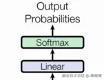
5.2.1 线性层的作用
- 通过对上一步的线性变化得到指定维度的输出, 也就是转换维度的作用.
5.2.2 softmax层的作用
- 使最后一维的向量中的数字缩放到0-1的概率值域内, 并满足他们的和为1.
5.2.3 线性层和softmax层的代码分析
ruby
# 解码器类 Generator 实现思路分析
# init函数 (self, d_model, vocab_size)
    # 定义线性层self.project
# forward函数 (self, x)
    # 数据 F.log_softmax(self.project(x), dim=-1)

class Generator(nn.Module):
    def __init__(self, d_model, vocab_size):
        # 参数d_model 线性层输入特征尺寸大小
        # 参数vocab_size 线层输出尺寸大小
        super(Generator, self).__init__()
        # 定义线性层
        self.project = nn.Linear(d_model, vocab_size)

    def forward(self, x):
        # 数据经过线性层 最后一个维度归一化 log方式
        x = F.log_softmax(self.project(x), dim=-1)
return x- nn.Linear演示:
ini
>>> m = nn.Linear(20, 30)
>>> input = torch.randn(128, 20)
>>> output = m(input)
>>> print(output.size())
torch.Size([128, 30])
6. 完整Transformer模型
将编码器和解码器组合成完整的Transformer模型:
完整的Transformer模型可以表示为:
Transformer(X,Y)=Decoder(Encoder(X),Y)
python
class MyTransform(nn.Module):
    """
    Transformer模型实现
    包含编码器和解码器两部分
    """
    def __init__(self, heads, embed_dim, feed_hidden_size, dropout_p=0.1):
        """
        初始化Transformer模型

        Args:
            heads: 注意力头数
            embed_dim: 嵌入维度
            feed_hidden_size: 前馈网络隐藏层大小
            dropout_p: dropout概率
        """
        super().__init__()

        # 创建编码器层模板
        encoder_layer = EncoderLayer(heads=heads, embed_dim=embed_dim,
                                     hidden_size=feed_hidden_size, dropout_p=dropout_p)
        # 创建包含6层的编码器
        self.encoder = Encoder(layer=encoder_layer, N=6, embed_dim=embed_dim)

        # 创建解码器层模板
        decoder_layer = DecoderLayer(heads=heads, embed_dim=embed_dim,
                                     feed_forward_hidden_size=feed_hidden_size, dropout_p=dropout_p)

        # 创建包含6层的解码器
        self.decoder = Decoder(decoder_layer=decoder_layer, n=6, embed_dim=embed_dim)

    def forward(self, x, y, target_mask, source_mask):
        """
        前向传播

        Args:
            x: 源序列输入 [batch_size, src_seq_len, embed_dim]
            y: 目标序列输入 [batch_size, tgt_seq_len, embed_dim]
            target_mask: 目标序列掩码(防止未来信息泄露)
            source_mask: 源序列掩码

        Returns:
            torch.Tensor: 解码器输出 [batch_size, tgt_seq_len, embed_dim]
        """
        # 编码器处理源序列
        encoder_output = self.encoder(x, source_mask)

        # 解码器处理目标序列,使用编码器输出作为键和值
        decoder_output = self.decoder(y, encoder_output, encoder_output, target_mask)

        return decoder_output
7. 公式与代码实现对照详解
为了更好地理解Transformer中各公式的实现,我们在此详细对照每个重要公式与其对应的代码实现。
7.1 注意力机制公式对照
注意力机制的核心公式:
Attention(Q,K,V)=softmax(dk QKT)V
对应的代码实现:
python
def attention(q, k, v, mask=None, dropout=None):
    # 获取维度
    embed_dim = k.size(-1)

    # 计算 QK^T
    q_k = torch.matmul(q, k.transpose(-1,-2))

    # 缩放操作:除以 sqrt(d_k)
    attn_weight = q_k / math.sqrt(embed_dim)

    # 应用掩码(如果存在)
    if mask is not None:
        attn_weight = attn_weight.masked_fill(mask == 0, -1e9)

    # softmax归一化
    attn_weight = nn.functional.softmax(attn_weight, dim=-1)

    # 应用dropout(如果存在)
    if dropout is not None:
        attn_weight = dropout(attn_weight)

    # 乘以 V
    res = torch.matmul(attn_weight , v)

    return res, attn_weight
7.2 多头注意力公式对照
多头注意力机制的公式:
MultiHead(Q,K,V)=Concat(head1,...,headh)WO
whereheadi=Attention(QWiQ,KWiK,VWiV)
对应的代码实现(MultiHeadAttention类的forward方法):
python
def forward(self, q, k, v, mask=None):
    if mask is not None:
        # 扩展mask的维度以匹配多头
        mask = mask.unsqueeze(0)

    batch_size = q.size(0)
    heads = self.heads
    embed_dim = q.size(-1)
    d_k = self.d_k

    # 对Q、K、V分别应用线性变换,然后reshape为(batch_size, heads, seq_len, d_k)
    q, k, v = [linear(x)
                .view(batch_size, -1, heads, d_k)
                .transpose(1,2)
                for linear,x in zip(self.linears,(q,k,v))]

    # 获取注意力机制输出
    output, attn_weight = attention(q, k, v, mask, self.dropout)

    # 合并多头到一个量中
    # 交换维度并合并heads和d_k维度
    res = output.transpose(1,2).contiguous().view(batch_size, -1, embed_dim)

    # 最后使用线性层做收尾处理
    return self.linears[-1](res)
7.3 位置编码公式对照
位置编码的公式:
PE(pos,2i)=sin(100002i/dmodelpos)
PE(pos,2i+1)=cos(100002i/dmodelpos)
对应的代码实现(PositionalEmbedding类的__init__方法):
python
def __init__(self, max_length, embed_dim, dropout_p=0.1):
    super().__init__()
    self.max_length = max_length
    self.embed_dim = embed_dim

    # Dropout层用于防止过拟合
    self.dropout = nn.Dropout(p=dropout_p)

    # 创建位置编码矩阵 [max_length, embed_dim]
    pe = torch.zeros(max_length, embed_dim)

    # 生成位置信息 [max_length, 1]
    pos = torch.arange(0, max_length).unsqueeze(1)

    # 生成维度索引 0, 2, 4, ..., embed_dim-2 (只取偶数索引)
    tow_i = torch.arange(0, embed_dim, 2)

    # 计算角度频率参数
    tmp_v = torch.exp((math.log(10000) * -tow_i / self.embed_dim))

    # 计算角度值:pos * 角度频率
    fn_v = tmp_v * pos

    # 偶数位置使用sin编码
    pe[:, 0::2] = torch.sin(fn_v)
    # 奇数位置使用cos编码
    pe[:, 1::2] = torch.cos(fn_v)

    # 增加batch维度 [1, max_length, embed_dim]
    pe = pe.unsqueeze(0)

    # 注册为buffer,不会被更新,但会随模型保存和加载
    self.register_buffer('pe', pe)
7.4 层归一化公式对照
层归一化的公式:
μ=H1∑i=1Hxi
σ2=H1∑i=1H(xi−μ)2
y=σ2+ϵ x−μ⊙γ+β
对应的代码实现(LayerNorm类的forward方法):
python
def forward(self, x):
    # 计算平均数
    x_mean = torch.mean(x, keepdim=True, dim=-1)

    # 计算标准差
    x_std = torch.std(x, keepdim=True, dim=-1)

    # 计算 (x-平均数) / (标准差+eps) = 标准化后的x
    res = (x - x_mean) / (x_std + self.eps)

    # 返回 W * x + b,应用可学习的缩放和偏移
    return self.w * res + self.b
7.5 前馈网络公式对照
前馈网络的公式:
FFN(x)=max(0,xW1+b1)W2+b2
对应的代码实现(FeedForward类的forward方法):
python
def forward(self, x):
    # 第一层线性变换: xW_1 + b_1
    x = self.linear1(x)

    # ReLU激活: max(0, xW_1 + b_1)
    x = self.relu(x)

    # Dropout防止过拟合
    x = self.dropout(x)

    # 第二层线性变换: max(0, xW_1 + b_1)W_2 + b_2
    x = self.linear2(x)

    return x
7.6 子层连接公式对照
子层连接的公式:
SublayerConnection(x,Sublayer)=LayerNorm(x+Dropout(Sublayer(x)))
对应的代码实现(SubLayers类的forward方法):
python
def forward(self, x, layer_fn):
    # 对输入应用指定的层函数,然后进行层归一化和dropout
    # 最后与原始输入进行残差连接(x + res)
    res  = self.dropout(self.norm(layer_fn(x)))
    return x + res
7.7 编码器层公式对照
编码器层的公式:
EncoderLayer(x)=SublayerConnection(SublayerConnection(x,SelfAttention),FFN)
对应的代码实现(EncoderLayer类的forward方法):
python
def forward(self, x, mask=None):
    # 第一层:自注意力机制
    x = self.layers[0](x, lambda x: self.multi_head_attn(x, x, x, mask))

    # 第二层:前馈神经网络
    x = self.layers[1](x, self.feed_ward)

    return x
7.8 解码器层公式对照
解码器层的公式:
DecoderLayer(x,encout)=SublayerConnection(SublayerConnection(SublayerConnection(x,MaskedSelfAttention),EncoderAttention),FFN)
对应的代码实现(DecoderLayer类的forward方法):
python
def forward(self, q, k, v, target_mask=None, source_mask=None):
    # 第一层:目标序列的自注意力(使用target_mask防止看到未来信息)
    res_1 = self.layers[0](q, lambda x: self.multi_head_attn(x, x, x, target_mask))

    # 第二层:编码器-解码器注意力(查询来自前一层,键值来自编码器输出)
    res_2 = self.layers[1](res_1, lambda x: self.multi_head_attn(x, k, v, source_mask))

    # 第三层:前馈神经网络
    res_3 = self.layers[2](res_2, self.feed_forward)

    return res_3
7.9 完整Transformer模型公式对照
完整Transformer模型的公式:
Transformer(X,Y)=Decoder(Encoder(X),Y)
对应的代码实现(MyTransform类的forward方法):
python
def forward(self, x, y, target_mask, source_mask):
    # 编码器处理源序列
    encoder_output = self.encoder(x, source_mask)

    # 解码器处理目标序列,使用编码器输出作为键和值
    decoder_output = self.decoder(y, encoder_output, encoder_output, target_mask)

    return decoder_output
8. 辅助函数
一些辅助函数帮助构建模型:
python
def clone_modules(module, N):
    """
    克隆N个相同的模块

    Args:
        module: 要克隆的模块
        N: 克隆的数量

    Returns:
        nn.ModuleList: 包含N个相同模块的列表
    """
    return nn.ModuleList(copy.deepcopy(module) for _ in range(N))

def get_mask(size):
    """
    生成上三角掩码矩阵,用于防止未来信息泄露(在解码器中使用)

    Args:
        size: 掩码矩阵的尺寸 (heads, seq_len, seq_len)

    Returns:
        torch.Tensor: 上三角为0,下三角和对角线为1的掩码矩阵
    """
    tensor = torch.ones(size=size, dtype=torch.long)
    # triu生成上三角矩阵,k=1表示对角线上方的元素为1,其余为0
    # 1-操作将其反转,使对角线和下三角为1,上三角为0
    return 1-torch.triu(tensor, 1)
9. 测试代码
测试模型各部分功能:
python
def test_transform():
    """
    测试完整的Transformer模型
    """
    # 占位符,无实际作用
    pass

    # 创建测试源序列数据
    x = torch.tensor([
        [1, 2, 3, 4],
        [2, 4, 5, 6]
    ])
    embed_dim = 512
    # 创建嵌入序列模块
    embedding = EmbeddingSequential(1000, 512, 60)
    # 获取源序列嵌入表示
    embedding_x = embedding(x)
    print('EmbeddingSequential', embedding_x.shape)
    heads = 8
    # 生成源序列掩码
    source_mask = get_mask(size=(heads, x.size(-1), x.size(-1)))
    dropout_p = 0.1
    hidden_size = 2048

    # 创建目标序列数据
    y = torch.tensor([
        [1, 2, 3, 4, 5, 6],
        [2, 3, 4, 5, 6, 7]
    ])

    # 深拷贝嵌入模块处理目标序列
    embed_y = copy.deepcopy(embedding)(y)

    print('embed_y', embed_y)
    # 生成目标序列掩码
    target_mask = get_mask(size=(heads, y.size(-1), y.size(-1)))
    # 创建Transformer模型
    transformer = MyTransform(heads=heads, embed_dim=embed_dim, feed_hidden_size=hidden_size, dropout_p=dropout_p)

    # Transformer前向传播
    decoder_output = transformer(embedding_x, embed_y, target_mask, source_mask)

    # 创建生成器
    generator = Generator(embed_dim, output_size=2000)

    # 生成预测结果
    pre_v = generator(decoder_output)

    print('pre_v', pre_v)
10. 项目源码
本项目完整源码已开源,您可以在以下GitHub仓库中获取:
源码包含了完整的Transformer实现,以及详细的中文注释,方便学习和理解。项目结构如下:
bash
transformer-implementation/
├── common.py              # 公共组件:注意力机制、多头注意力、层归一化等
├── encoder_module.py      # 编码器模块实现
├── decoder_module.py      # 解码器模块实现
├── embeddings.py          # 词嵌入和位置编码实现
├── generator.py           # 输出生成器
├── transform.py           # Transformer模型主体
└── test.py               # 测试代码
您可以通过以下方式使用该项目:
bash
git clone https://github.com/KobeCYL/transformer-implementation.git
cd transformer-implementation
python test.py
欢迎提交Issue和Pull Request,共同完善这个教学用途的Transformer实现。
11. 总结
通过手写Transformer的实现,我们可以更深入地理解其内部工作机制:
- 注意力机制:核心组件,允许模型关注输入序列的不同部分
- 多头注意力:并行计算多个注意力表示,增强模型的表达能力
- 位置编码:为模型提供序列顺序信息
- 残差连接和层归一化:稳定训练过程,加速收敛
- 前馈网络:对每个位置的表示进行非线性变换
Transformer的这些设计使其能够并行处理序列数据,有效捕获长距离依赖关系,成为现代NLP模型的基础架构。通过手动实现这些组件,我们不仅加深了对Transformer架构的理解,也为后续的模型改进和优化奠定了基础。
12. 关注我们
如果你觉得这篇文章对你有帮助,欢迎:
- 点赞支持:如果内容对你有帮助,请不要吝啬你的赞👍
- 分享传播:将文章分享给更多需要的朋友,让知识传递更远
- 关注作者:关注我的GitHub和博客,获取更多深度学习和自然语言处理的干货内容
- 评论交流:在评论区留下你的想法和问题,我们一起讨论学习
更多关于Transformer、BERT、GPT等前沿NLP技术的深度解析,敬请关注!
- GitHub: [github.com/KobeCYL/tra...](https://link.juejin.cn?target=https%3A%2F%2Fgithub.com%2FKobeCYL%2Ftransformer-implementation.git "https://github.com/KobeCYL/transformer-implementation.git")
- 知乎专栏: [juejin.cn/column/7564...](https://juejin.cn/column/7564951282625134602 "https://juejin.cn/column/7564951282625134602")
- 微信公众号: 小果的迭代人生
让我们一起在AI的道路上不断前行,探索更多技术的奥秘!🚀