
二维平面上,2个雷达观测一个目标,雷达仅观测与UKF滤波后的效果对比。同时输出轨迹、定位误差、误差统计特性等。 软件环境:MATLAB R2016b 或更高版本
文章目录
程序简介
本代码实现了一个基于**无迹卡尔曼滤波器(Unscented Kalman Filter, UKF)**的多雷达目标跟踪系统。系统能够融合多个雷达的观测数据(距离和方位角),对二维平面上的机动目标进行高精度状态估计和轨迹跟踪。
核心功能
无迹卡尔曼滤波(UKF)
- 采用无迹变换(Unscented Transform)处理非线性观测模型
- 通过Sigma点采样准确传播均值和协方差
- 相比扩展卡尔曼滤波(EKF),无需计算雅可比矩阵
- 对强非线性系统具有更高的估计精度(泰勒展开精度达3阶)
多雷达数据融合
- 支持多个雷达站的协同观测
- 采用序贯更新策略融合不同雷达的观测数据
- 自动处理雷达检测概率和观测丢失情况
- 充分利用空间分集提高跟踪精度
机动目标跟踪
- 采用匀速(CV)运动模型作为基础
- 能够跟踪包含转弯、加速等机动动作的目标
- 通过过程噪声建模适应目标机动
参数调整
代码中所有标注 【可修改】 的参数都可以根据实际需求调整:
- 基本参数:采样周期、仿真时间
- 雷达配置:雷达位置、数量、探测距离
- 噪声参数:测量噪声、过程噪声标准差
- 初始状态:初始位置、速度估计及不确定性
- UKF参数:α、β、κ(影响Sigma点分布)
算法优势
UKF vs EKF的对比表格:
| 特性 | UKF | EKF |
|---|---|---|
| 线性化方法 | 无迹变换(统计线性化) | 雅可比矩阵(一阶泰勒展开) |
| 精度阶数 | 3阶 | 2阶 |
| 是否需要求导(雅克比) | 否 | 是 |
| 非线性适应性 | 强 | 中 |
| 计算复杂度 | 中等(2n+1次函数调用) | 较低 |
| 数值稳定性 | 好 | 中 |
适合UKF的场景:
- 观测模型高度非线性(如极坐标观测)
- 状态转移模型复杂
- 难以求解雅可比矩阵
- 对精度要求高
⚠️ 可用EKF的场景:
- 弱非线性系统
- 计算资源受限
- 对实时性要求极高
运行结果
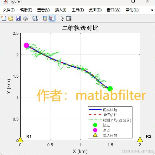
轨迹图,包含真值、仅雷达观测、UKF滤波估计后:
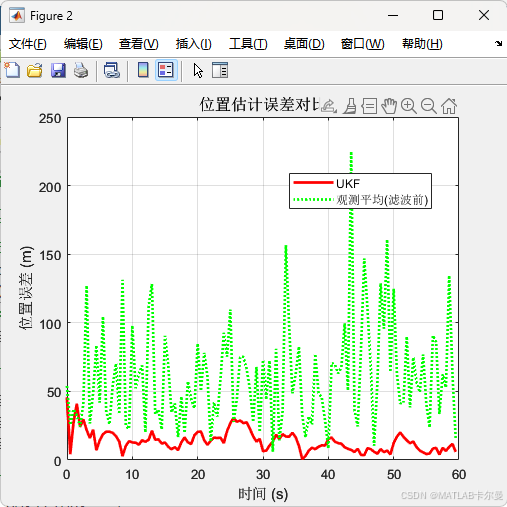
误差对比:
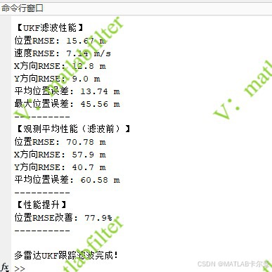
统计特性输出:
MATLAB源代码
部分代码:
matlab
% 2雷达二维目标跟踪滤波系统 - UKF实现,匀速运动模型
% 输入:雷达观测数据(距离、方位角),输出:目标状态估计(位置、速度)
% 作者: matlabfilter
% 2025-11-09/Ver1
clc; clear; close all;
rng(0);
%% === 系统参数配置 ===
config = struct();
% 【可修改】基本参数
config.T = 0.5; % 采样周期 (s) - 可修改
config.total_time = 60; % 总仿真时间 (s) - 可修改
config.num_steps = config.total_time / config.T;
% 【可修改】雷达位置配置 [x, y] (m) - 固定位置,需要时可修改
radar_positions = [
0, 0; % 雷达1位置
2000, 0]; % 雷达2位置
% 【可修改】测量噪声标准差 - 根据实际雷达精度调整
config.sigma_range = 20; % 距离测量噪声标准差 (m)
config.sigma_bearing = 0.05; % 方位角测量噪声标准差 (rad) ≈ 2.86°
% 【可修改】过程噪声标准差 - 影响滤波器的跟踪能力
config.sigma_acc = 2.0; % 加速度过程噪声标准差 (m/s²)
% 【可修改】仿真参数
config.detection_prob = 0.95; % 检测概率 - 可调整丢失观测的概率
config.max_range = 15000; % 雷达最大探测距离 (m)
% 【新增】UKF参数
config.alpha = 1e-3; % Sigma点分布参数 (通常1e-4到1)
config.beta = 2; % 高斯分布最优值为2
config.kappa = 0; % 次级缩放参数 (通常为0或3-n)
%% === 初始化UKF滤波器 ===
% 状态向量: [x, y, vx, vy]'
% x,y: 位置 (m), vx,vy: 速度 (m/s)
% 二维轨迹对比(主图)
figure;
plot(true_traj(1,:)/1000, true_traj(2,:)/1000, 'b-', 'LineWidth', 2.5, 'DisplayName', '真实轨迹');
hold on;
plot(est_traj(1,:)/1000, est_traj(2,:)/1000, 'r--', 'LineWidth', 2, 'DisplayName', 'UKF估计');
plot(obs_only(1,:)/1000, obs_only(2,:)/1000, 'g:', 'LineWidth', 1.5, 'DisplayName', '观测平均(滤波前)');
% 标记起点和终点
plot(true_traj(1,1)/1000, true_traj(2,1)/1000, 'go', ...
'MarkerSize', 12, 'MarkerFaceColor', 'g', 'DisplayName', '起点');
plot(true_traj(1,end)/1000, true_traj(2,end)/1000, 'mo', ...
'MarkerSize', 12, 'MarkerFaceColor', 'm', 'DisplayName', '终点');
% 绘制雷达位置
for r = 1:size(radar_pos, 1)
if r == 1
plot(radar_pos(r,1)/1000, radar_pos(r,2)/1000, ...
'^k', 'MarkerSize', 12, 'MarkerFaceColor', 'yellow', 'DisplayName', '雷达位置');
else
plot(radar_pos(r,1)/1000, radar_pos(r,2)/1000, ...
'^k', 'MarkerSize', 12, 'MarkerFaceColor', 'yellow', 'HandleVisibility', 'off');
end
text(radar_pos(r,1)/1000 + 0.1, radar_pos(r,2)/1000 + 0.1, ...
sprintf('R%d', r), 'FontSize', 10, 'FontWeight', 'bold');
end
xlabel('X (km)', 'FontSize', 12);
ylabel('Y (km)', 'FontSize', 12);
title('二维轨迹对比', 'FontSize', 14, 'FontWeight', 'bold');
legend('Location', 'best');
grid on;
% 位置误差对比
figure;
position_error_ukf = sqrt(sum(errors(1:2,:).^2, 1));
position_error_obs = sqrt(sum((obs_only - true_traj(1:2,:)).^2, 1));
plot(time_vec, position_error_ukf, 'r-', 'LineWidth', 2, 'DisplayName', 'UKF');
hold on;
plot(time_vec, position_error_obs, 'g:', 'LineWidth', 2, 'DisplayName', '观测平均(滤波前)');
xlabel('时间 (s)', 'FontSize', 11);
ylabel('位置误差 (m)', 'FontSize', 11);
title('位置估计误差对比', 'FontSize', 12);
legend('Location', 'best');
grid on;
figure;
plot(time_vec, errors(1,:), 'r-', 'LineWidth', 1.5, 'DisplayName', 'X轴(UKF)'); hold on;
plot(time_vec, errors(2,:), 'b-', 'LineWidth', 1.5, 'DisplayName', 'Y轴(UKF)');
plot(time_vec, obs_only(1,:) - true_traj(1,:), 'r:', 'LineWidth', 1.5, 'DisplayName', 'X轴(观测)');
plot(time_vec, obs_only(2,:) - true_traj(2,:), 'b:', 'LineWidth', 1.5, 'DisplayName', 'Y轴(观测)');
xlabel('时间 (s)', 'FontSize', 11);
ylabel('误差 (m)', 'FontSize', 11);
title('各轴位置误差分量对比', 'FontSize', 12);
legend('Location', 'best');
grid on;
% 作者: matlabfilter
figure;
velocity_error = sqrt(sum(errors(3:4,:).^2, 1));
plot(time_vec, velocity_error, 'g-', 'LineWidth', 2);
xlabel('时间 (s)', 'FontSize', 11);
ylabel('速度误差 (m/s)', 'FontSize', 11);
title('速度估计误差(仅UKF)', 'FontSize', 12);
grid on;
% 速度对比和协方差
figure;
true_speed = sqrt(sum(true_traj(3:4,:).^2, 1));
est_speed = sqrt(sum(est_traj(3:4,:).^2, 1));
plot(time_vec, true_speed, 'b-', 'LineWidth', 2, 'DisplayName', '真实速度'); hold on;
plot(time_vec, est_speed, 'r--', 'LineWidth', 2, 'DisplayName', 'UKF估计');
xlabel('时间 (s)', 'FontSize', 11);
ylabel('速度大小 (m/s)', 'FontSize', 11);
title('速度估计对比', 'FontSize', 12);
legend('Location', 'best');
grid on;
figure;
semilogy(time_vec, cov_trace, 'Color', [0.8, 0.4, 0], 'LineWidth', 2);
xlabel('时间 (s)', 'FontSize', 11);
ylabel('协方差迹', 'FontSize', 11);
title('滤波器不确定性变化', 'FontSize', 12);
grid on;
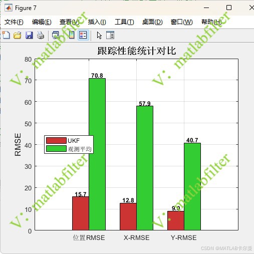
% 性能统计对比
figure;
rmse_pos_ukf = sqrt(mean(sum(errors(1:2,:).^2, 1)));
rmse_pos_obs = sqrt(mean(sum((obs_only - true_traj(1:2,:)).^2, 1)));
rmse_vel = sqrt(mean(sum(errors(3:4,:).^2, 1)));
rmse_x_ukf = sqrt(mean(errors(1,:).^2));
rmse_y_ukf = sqrt(mean(errors(2,:).^2));
rmse_x_obs = sqrt(mean((obs_only(1,:) - true_traj(1,:)).^2));
rmse_y_obs = sqrt(mean((obs_only(2,:) - true_traj(2,:)).^2));
% 创建对比数据
categories = {'位置RMSE', 'X-RMSE', 'Y-RMSE'};
ukf_data = [rmse_pos_ukf, rmse_x_ukf, rmse_y_ukf];
obs_data = [rmse_pos_obs, rmse_x_obs, rmse_y_obs];
x_pos = 1:length(categories);
bar_width = 0.35;
b1 = bar(x_pos - bar_width/2, ukf_data, bar_width, 'FaceColor', [0.8, 0.2, 0.2], 'DisplayName', 'UKF');
hold on;
b2 = bar(x_pos + bar_width/2, obs_data, bar_width, 'FaceColor', [0.2, 0.8, 0.2], 'DisplayName', '观测平均');
set(gca, 'XTick', x_pos);
set(gca, 'XTickLabel', categories);
ylabel('RMSE', 'FontSize', 12);
title('跟踪性能统计对比', 'FontSize', 14, 'FontWeight', 'bold');
legend('Location', 'best');
grid on;
% 作者: matlabfilter
% 添加数值标签
for i = 1:length(ukf_data)
if ~isnan(ukf_data(i))
text(x_pos(i) - bar_width/2, ukf_data(i) + max([ukf_data, obs_data])*0.02, ...
sprintf('%.1f', ukf_data(i)), ...
'HorizontalAlignment', 'center', 'FontWeight', 'bold', 'FontSize', 9);
end
if ~isnan(obs_data(i))
text(x_pos(i) + bar_width/2, obs_data(i) + max([ukf_data, obs_data])*0.02, ...
sprintf('%.1f', obs_data(i)), ...
'HorizontalAlignment', 'center', 'FontWeight', 'bold', 'FontSize', 9);
end
end
% 打印详细统计结果
fprintf('\n=== 跟踪性能统计 ===\n');
fprintf('滤波算法: 无迹卡尔曼滤波 (UKF)\n');
fprintf('观测类型: 距离 + 方位角 (2D)\n');
fprintf('雷达数量: %d\n', 2);
fprintf('----------\n');
fprintf('【UKF滤波性能】\n');
fprintf('位置RMSE: %.2f m\n', rmse_pos_ukf);
fprintf('速度RMSE: %.2f m/s\n', rmse_vel);
fprintf('X方向RMSE: %.1f m\n', rmse_x_ukf);
fprintf('Y方向RMSE: %.1f m\n', rmse_y_ukf);
fprintf('平均位置误差: %.2f m\n', mean(sqrt(sum(errors(1:2,:).^2, 1))));
fprintf('最大位置误差: %.2f m\n', max(sqrt(sum(errors(1:2,:).^2, 1))));
fprintf('----------\n');
fprintf('【观测平均性能(滤波前)】\n');
fprintf('位置RMSE: %.2f m\n', rmse_pos_obs);
fprintf('X方向RMSE: %.1f m\n', rmse_x_obs);
fprintf('Y方向RMSE: %.1f m\n', rmse_y_obs);
fprintf('平均位置误差: %.2f m\n', mean(sqrt(sum((obs_only - true_traj(1:2,:)).^2, 1))));
fprintf('----------\n');
fprintf('【性能提升】\n');
fprintf('位置RMSE改善: %.1f%%\n', 100*(rmse_pos_obs - rmse_pos_ukf)/rmse_pos_obs);
fprintf('----------\n');
end完整代码:
https://download.csdn.net/download/callmeup/92270215
扩展方向
可能的改进:
-
交互式多模型(IMM) :融合多个运动模型应对复杂机动
相关专栏:https://blog.csdn.net/callmeup/article/details/143357315?spm=1011.2415.3001.5331
-
自适应UKF :动态调整噪声协方差
-
平方根UKF(SR-UKF) :进一步提高数值稳定性
https://blog.csdn.net/callmeup/article/details/144522811?spm=1011.2415.3001.5331
如需帮助,或有导航、定位滤波相关的代码定制需求,请点击下方卡片联系作者