文章目录
摘要
本周学习了扩散模型,重温之前的扩散模型的知识和流程,并且对其中一些疑惑的点进行学习,通过代码生成了几张手写数字识别的数据集;也进行了对rcnn的代码学习,但是还没有攻克这个难题。
Abstract
This week, I studied diffusion models, revisited previous knowledge and processes of diffusion models, and studied some points that I was confused about. I generated several images of a handwritten digit recognition dataset through code; I also studied the RCNN code, but I haven't yet overcome this challenge.
1 Diffusion Model
最近的扩散模型很火,我之前也有对扩散模型进行过学习,但是当时还没有学习是很宽泛的,所以现在重新对扩散模型进行学习,温故而知新,并且借助pytorch,实现了一个简单的扩散模型,用于生成手写数字识别的训练样本。
要让机器学习可以预测一张图片,什么都没有,机器是不知道如何预测的,没有一个方向指引。扩散模型是将一张图片进行随机时间步的加入高斯噪声,让后让模型去噪来学习图片的像素分布,这个时候的扩散模型没有约束控制,只能生成和训练图像分布类似的图像。
1.1 前向过程
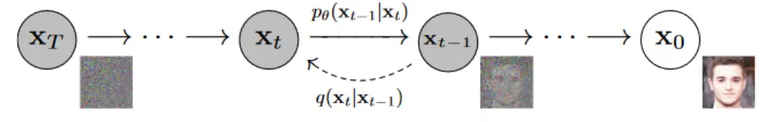
从 x 0 x_0 x0到 x T x_T xT的过程就是前向加噪过程,对原始图片 x 0 x_0 x0进行操作,使其变得模糊,去噪就类似还原过程。
论文中加入的噪声是正态分布的。往图片加入噪声,图片就会变得很模糊接近纯噪声,纯噪声代表多样性,去噪时会产生更多样的图片。
x 0 x_0 x0是原始图片,其满足初始分布 q ( x 0 ) q(x_0) q(x0),即 x 0 − q ( x 0 ) x_0-q(x_0) x0−q(x0)
对于 t ∈ 1 , T t\in 1,T t∈1,T时刻, x t x_t xt和 x t − 1 x_{t-1} xt−1满足如下关系
x t = 1 − β t x t − 1 + β t ϵ x_t=\sqrt{1-\beta_t}x_{t-1}+\sqrt{\beta_t}\epsilon xt=1−βt xt−1+βt ϵ
ϵ ∼ N ( 0 , 1 ) \epsilon \sim N(0,1) ϵ∼N(0,1)
令 α t = 1 − β t \alpha_t=1-\beta_t αt=1−βt,则公式变形为
x t = α t x t − 1 + 1 − α t ϵ x_t=\sqrt{\alpha_t}x_{t-1}+\sqrt{1-\alpha_t}\epsilon xt=αt xt−1+1−αt ϵ
其中的 β t \beta_t βt是常数,取值是0.0001,0.02的线性插值。
x t = α t x t − 1 + 1 − α t ϵ = α t ( α t − 1 x t − 2 + 1 − α t − 1 ϵ ) + 1 − α t ϵ = α t α t − 1 x t − 2 + α t 1 − α t − 1 + 1 − α t ϵ x_t =\sqrt{\alpha_t}x_{t-1}+\sqrt{1-\alpha_t}\epsilon =\sqrt{\alpha_t}(\sqrt{\alpha_{t-1}}x_{t-2}+\sqrt{1-\alpha_{t-1}}\epsilon )+\sqrt{1-\alpha_t}\epsilon \\ = \sqrt{\alpha_t\alpha_{t-1}}x_{t-2}+\sqrt{\alpha_t}\sqrt{1-\alpha_{t-1}}+\sqrt{1-\alpha_t}\epsilon xt=αt xt−1+1−αt ϵ=αt (αt−1 xt−2+1−αt−1 ϵ)+1−αt ϵ=αtαt−1 xt−2+αt 1−αt−1 +1−αt ϵ
由正态分布的叠加性, α t 1 − α t − 1 ϵ + 1 − α t ϵ \sqrt{\alpha_t}{\sqrt {1-\alpha_{t-1}}}\epsilon+\sqrt{1-\alpha_t}\epsilon αt 1−αt−1 ϵ+1−αt ϵ可以看作
X 1 ∼ α t 1 − α t − 1 θ = N ( 0 , α t ( 1 − α t − 1 ) ) X 2 ∼ 1 − α t θ = N ( 0 , 1 − α t ) X 1 + X 2 = N ( 0 , 1 − α t α t − 1 ) \begin{aligned}X_1 \sim \sqrt{\alpha_t}\sqrt{1-\alpha_{t-1}}\theta &=N(0,\alpha_t(1-\alpha_{t-1}))\\ X_2 \sim \sqrt{1-\alpha_t}\theta &=N(0,1-\alpha_t) \\ X_1+X_2&=N(0,1-\alpha_t\alpha_{t-1})\end{aligned} X1∼αt 1−αt−1 θX2∼1−αt θX1+X2=N(0,αt(1−αt−1))=N(0,1−αt)=N(0,1−αtαt−1)
公式则化简为 x t = α t α t − 1 x t − 2 + ( 1 − α t α t − 1 ) ϵ x_t=\sqrt{\alpha_t\alpha_{t-1}}x_{t-2}+(\sqrt{1-\alpha_t\alpha_{t-1}})\epsilon xt=αtαt−1 xt−2+(1−αtαt−1 )ϵ
由数学归纳法,可以进一步推导得 x t = α t α t − 1 . . . α 1 x 0 + ( 1 − α t α t − 1 α 1 ) ϵ x_t = \sqrt{\alpha_t\alpha_{t-1}...\alpha_1}x_{0} + (\sqrt{1-\alpha_t\alpha_{t-1}\alpha_{1}})\epsilon xt=αtαt−1...α1 x0+(1−αtαt−1α1 )ϵ
令 α ˉ t = α t α t − 1 ⋯ α 1 \bar\alpha_t=\alpha_t\alpha_{t-1}\cdots \alpha_1 αˉt=αtαt−1⋯α1,则公式简化为 x t = α t ˉ x 0 + 1 − α t ˉ ϵ x_t = \sqrt{\bar{\alpha_t}}x_0 + \sqrt{1-\bar{\alpha_t}}\epsilon xt=αtˉ x0+1−αtˉ ϵ
x t = α t ˉ x 0 + 1 − α t ˉ ϵ x_t = \sqrt{\bar{\alpha_t}}x_0 + \sqrt{1-\bar{\alpha_t}}\epsilon xt=αtˉ x0+1−αtˉ ϵ可以求出 x 0 x_0 x0的表达式为 x 0 = x t − 1 − α ˉ t ϵ α ˉ t x_0=\frac{x_t-\sqrt{1-\bar \alpha_t}\epsilon}{\sqrt{\bar \alpha_t}} x0=αˉt xt−1−αˉt ϵ
公式化简后发现 x t x_t xt只和 x 0 x_0 x0及 α \alpha α有关,不需要进行多次迭代。
由于 β t \beta_t βt一直在变大,则 α t \alpha_t αt一直在变小,则当 t → T , α ˉ T → 0 t\rightarrow T,\bar \alpha_T\rightarrow 0 t→T,αˉT→0,则 x T → ϵ x_T\rightarrow \epsilon xT→ϵ
在前向加噪的过程,进行非常多的步骤的时候(例如T=1000),最终产生的图片 x T x_T xT接近于高斯分布。
在之前,我认为是需要对所有的图片都进行1000步加噪,然后让模型去噪。这是我当时理解错误了,其实是对每一张图片随机的加噪,这样的差异,才会让模型学习到原始图片的分布。
1.2反向去噪
最后的噪声图片 x T x_T xT来自高斯分布
去噪过程中不知道上一时刻 x t − 1 x_{t-1} xt−1的值,是需要用 x t x_t xt进行预测,所以只能用概率的形式,采用贝叶斯公式取尖酸后验概率 P ( x t − 1 ∣ x t ) P(x_{t-1}|x_t) P(xt−1∣xt)
P ( x t − 1 ∣ x t ) = P ( x t − 1 x t ) P ( x t ) = P ( x t ∣ x t − 1 ) P ( x t − 1 ) P ( x t ) P(x_{t-1}|x_t) = \frac{P(x_{t-1}x_t)}{P(x_t)} = \frac{P(x_t|x_{t-1})P(x_{t-1})}{P(x_t)} P(xt−1∣xt)=P(xt)P(xt−1xt)=P(xt)P(xt∣xt−1)P(xt−1)
在已知原图 x 0 x_0 x0的情况下,进行公式改写
P ( x t − 1 ∣ x t , x 0 ) = P ( x t ∣ x t − 1 , x 0 ) P ( x t − 1 ∣ x 0 ) P ( x t ∣ x 0 ) P(x_{t-1}|x_t,x_0) = \frac{P(x_t|x_{t-1},x_0)P(x_{t-1}|x_0)}{P(x_t|x_0)} P(xt−1∣xt,x0)=P(xt∣x0)P(xt∣xt−1,x0)P(xt−1∣x0)
等式右边部分都变成先验概率,由 x t = α t ˉ x 0 + 1 − α t ˉ ϵ x_t = \sqrt{\bar{\alpha_t}}x_0 + \sqrt{1-\bar{\alpha_t}}\epsilon xt=αtˉ x0+1−αtˉ ϵ和 x t = 1 − β t x t − 1 + β t ϵ x_t = \sqrt{1-\beta_t}x_{t-1} + \sqrt{\beta_t}\epsilon xt=1−βt xt−1+βt ϵ
P ( x t − 1 ∣ x t , x 0 ) = N ( α t x t − 1 , 1 − α t ) N ( α t − 1 ˉ x 0 , 1 − α t − 1 ˉ ) N ( α t ˉ x 0 , 1 − α t ˉ ) P(x_{t-1}|x_t,x_0) = \frac{N(\sqrt{\alpha_t}x_{t-1},1-\alpha_t) N(\sqrt{\bar{\alpha_{t-1}}}x_0,1-\bar{\alpha_{t-1}})}{N(\sqrt{\bar{\alpha_{t}}}x_0,1-\bar{\alpha_{t}})} P(xt−1∣xt,x0)=N(αtˉ x0,1−αtˉ)N(αt xt−1,1−αt)N(αt−1ˉ x0,1−αt−1ˉ)
展开
P ( x t − 1 ∣ x t , x 0 ) ∝ e x p − 1 2 ( x t − α t x t − 1 ) 2 1 − α t + ( x t − 1 − α t − 1 ˉ x 0 ) 2 1 − α t − 1 ˉ − ( x t − α t ˉ x 0 ) 2 1 − α t ˉ P(x_{t-1}|x_t,x_0) \propto exp -\frac{1}{2}\\frac{(x_t-\\sqrt{\\alpha_t}x_{t-1})\^2}{1-\\alpha_t} + \\frac{(x_{t-1}-\\sqrt{\\bar{\\alpha_{t-1}}}x_0)\^2}{1-\\bar{\\alpha_{t-1}}} - \\frac{(x_t-\\sqrt{\\bar{\\alpha_t}}x_0)\^2}{1-\\bar{\\alpha_t}} P(xt−1∣xt,x0)∝exp−211−αt(xt−αt xt−1)2+1−αt−1ˉ(xt−1−αt−1ˉ x0)2−1−αtˉ(xt−αtˉ x0)2
此时由于 x t − 1 x_{t-1} xt−1是关注的变量,所以整理成关于 x t − 1 x_{t-1} xt−1的形式
P ( x t − 1 ∣ x t , x 0 ) ∝ e x p − 1 2 ( α t 1 − α t + 1 1 − α t − 1 ˉ ) x t − 1 2 − ( 2 α t 1 − α t x t + 2 α t − 1 ˉ 1 − α t − 1 ˉ x 0 ) x t − 1 + C ( x t , x 0 ) P(x_{t-1}|x_t,x_0) \propto exp -\frac{1}{2}(\\frac{\\alpha_t}{1-\\alpha_t}+\\frac{1}{1-\\bar{\\alpha_{t-1}}})x_{t-1}\^2 - (\\frac{2\\sqrt{\\alpha_t}}{1-\\alpha_t}x_t+\\frac{2\\sqrt{\\bar{\\alpha_{t-1}}}}{1-\\bar{\\alpha_{t-1}}}x_0)x_{t-1} + C(x_t,x_0) P(xt−1∣xt,x0)∝exp−21(1−αtαt+1−αt−1ˉ1)xt−12−(1−αt2αt xt+1−αt−1ˉ2αt−1ˉ x0)xt−1+C(xt,x0)
其中 C ( x t , x 0 ) C(x_t,x_0) C(xt,x0)与 x t − 1 x_{t-1} xt−1无关,只影响前面的系数
标准正态分布满足 ∝ e x p − x 2 + μ 2 − 2 x μ 2 σ 2 \propto exp -\frac{x^2+\mu^2-2x\mu}{2\sigma^2} ∝exp−2σ2x2+μ2−2xμ,则
1 σ 2 = α t 1 − α t + 1 1 − α t − 1 ˉ = 1 − α t ˉ ( 1 − α t ) ( 1 − α t − 1 ˉ ) σ 2 = β t ( 1 − α t − 1 ˉ ) 1 − α t ˉ μ = 1 2 σ 2 ( 2 α t 1 − α t x t + 2 α t − 1 ˉ 1 − α t − 1 ˉ x 0 ) = α t − 1 ˉ ( 1 − α t ) 1 − α t ˉ x 0 + ( 1 − α t − 1 ˉ ) α t 1 − α t ˉ x t \begin{aligned}\frac{1}{\sigma^2} &= \frac{\alpha_t}{1-\alpha_t} + \frac{1}{1-\bar{\alpha_{t-1}}} = \frac{1-\bar{\alpha_t}}{(1-\alpha_t)(1-\bar{\alpha_{t-1}})} \\ \sigma^2 &= \frac{\beta_t(1-\bar{\alpha_{t-1}})}{1-\bar{\alpha_t}} \\ \mu &= \frac{1}{2}\sigma^2(\frac{2\sqrt{\alpha_t}}{1-\alpha_t}x_t+\frac{2\sqrt{\bar{\alpha_{t-1}}}}{1-\bar{\alpha_{t-1}}}x_0) = \frac{\sqrt{\bar{\alpha_{t-1}}}(1-\alpha_t)}{1-\bar{\alpha_t}}x_0 + \frac{(1-\bar{\alpha_{t-1}})\sqrt{\alpha_t}}{1-\bar{\alpha_{t}}}x_t \\ \end{aligned} σ21σ2μ=1−αtαt+1−αt−1ˉ1=(1−αt)(1−αt−1ˉ)1−αtˉ=1−αtˉβt(1−αt−1ˉ)=21σ2(1−αt2αt xt+1−αt−1ˉ2αt−1ˉ x0)=1−αtˉαt−1ˉ (1−αt)x0+1−αtˉ(1−αt−1ˉ)αt xt
又因为 x t = α t ˉ x 0 + 1 − α t ˉ ϵ x_t = \sqrt{\bar{\alpha_t}}x_0 + \sqrt{1-\bar{\alpha_t}}\epsilon xt=αtˉ x0+1−αtˉ ϵ,则可以将上式的 x 0 x_0 x0全部换掉
μ = 1 α t ( α t − α t ˉ 1 − α t ˉ x t + α t ˉ ( 1 − α t ) 1 − α t ˉ ∗ x t − 1 − α t ˉ ϵ α t ˉ ) = 1 α t α t − α t ˉ 1 − α t ˉ x t + 1 − α t 1 − α t ˉ ∗ ( x t − 1 − α t ˉ ϵ ) = 1 α t ( x t − 1 − α t 1 − α t ˉ 1 − α t ˉ ϵ ) = 1 α t ( x t − 1 − α t 1 − α t ˉ ϵ ) \begin{aligned}\mu &= \frac{1}{\sqrt{\alpha_t}}(\frac{\alpha_t-\bar{\alpha_t}}{1-\bar{\alpha_t}}x_t + \frac{\sqrt{\bar{\alpha_t}}(1-\alpha_t)}{1-\bar{\alpha_t}}*\frac{x_t-\sqrt{1-\bar{\alpha_t}}\epsilon}{\sqrt{\bar{\alpha_t}}}) \\ &= \frac{1}{\sqrt{\alpha_t}}\\frac{\\alpha_t-\\bar{\\alpha_t}}{1-\\bar{\\alpha_t}}x_t + \\frac{1-\\alpha_t}{1-\\bar{\\alpha_t}}\*(x_t-\\sqrt{1-\\bar{\\alpha_t}}\\epsilon) \\ &= \frac{1}{\sqrt{{\alpha_t}}}(x_t - \frac{1-\alpha_t}{1-\bar{\alpha_t}}\sqrt{1-\bar{\alpha_t}}\epsilon) \\ &= \frac{1}{\sqrt{\alpha_t}}(x_t - \frac{1-\alpha_t}{\sqrt{1-\bar{\alpha_t}}}\epsilon)\end{aligned} μ=αt 1(1−αtˉαt−αtˉxt+1−αtˉαtˉ (1−αt)∗αtˉ xt−1−αtˉ ϵ)=αt 11−αtˉαt−αtˉxt+1−αtˉ1−αt∗(xt−1−αtˉ ϵ)=αt 1(xt−1−αtˉ1−αt1−αtˉ ϵ)=αt 1(xt−1−αtˉ 1−αtϵ)
P ( x t − 1 ∣ x t ) = N ( 1 α t ( x t − 1 − α t 1 − α t ˉ ϵ ) , ( 1 − α t ) ( 1 − α t − 1 ˉ ) 1 − α t ˉ ) P(x_{t-1}|x_t) = N(\frac{1}{\sqrt{\alpha_t}}(x_t - \frac{1-\alpha_t}{\sqrt{1-\bar{\alpha_t}}}\epsilon),\frac{(1-\alpha_t)(1-\bar{\alpha_{t-1}})}{1-\bar{\alpha_t}}) P(xt−1∣xt)=N(αt 1(xt−1−αtˉ 1−αtϵ),1−αtˉ(1−αt)(1−αt−1ˉ))
以上只是简单的前向和反向的介绍,还有 ϵ \epsilon ϵ是未知的。
就是需要借助机器学习来你和最后的 P ( x t − 1 ∣ x t ) P(x_{t-1}|x_t) P(xt−1∣xt)。DDPM借助Unet模型来实现,Unet模型,在上一周的报告中已经陈述了。
1.3 代码
python
import math
import os

import torch
import torch.nn as nn
import torchvision
from PIL import Image
from matplotlib import pyplot as plt
from torch.utils.data import Dataset, DataLoader
from torchvision import transforms

torch.manual_seed(42)


class Attention(nn.Module):
    def __init__(self, d_k):
        super().__init__()
        self.d_k = d_k

    def forward(self, q, k, v):
        scores = torch.matmul(q, k.transpose(-1, -2)) / math.sqrt(self.d_k)
        attention_weights = torch.softmax(scores, dim=-1)
        attention = torch.matmul(attention_weights, v)
        return attention, attention_weights

class MultiHeadAttention(nn.Module):
    def __init__(self, d_model, num_heads):
        super().__init__()
        self.d_model = d_model
        self.num_heads = num_heads
        self.d_k = d_model // num_heads
        assert d_model % num_heads == 0, "向量大小与头数要整除"
        # 使用单个大线性层而不是多个小线性层
        self.w_q = nn.Linear(d_model, d_model)
        self.w_k = nn.Linear(d_model, d_model)
        self.w_v = nn.Linear(d_model, d_model)
        self.attention = Attention(self.d_k)
        self.linear = nn.Linear(d_model, d_model)
        self.attention_weights = None

    def forward(self, q, k, v):
        batch_size, seq_len = q.size(0), q.size(1)
        # 应用线性变换
        q = self.w_q(q)
        k = self.w_k(k)
        v = self.w_v(v)
        q = q.view(batch_size, seq_len, self.num_heads, self.d_k).transpose(1, 2)
        k = k.view(batch_size, seq_len, self.num_heads, self.d_k).transpose(1, 2)
        v = v.view(batch_size, seq_len, self.num_heads, self.d_k).transpose(1, 2)
        attention_output, self.attention_weights = self.attention(q, k, v)
        attention_output = attention_output.transpose(1, 2).contiguous().view(
            batch_size, seq_len, self.d_model)
        output = self.linear(attention_output)
        return output

def embed(t, d_model, max_len=1000):
    half = d_model // 2
    freqs = torch.exp(-math.log(max_len) * torch.arange(start=0, end=half, dtype=torch.float32) / half).to(
        device=t.device)
    args = t[:, None].float() * freqs[None]
    embedding = torch.cat([torch.cos(args), torch.sin(args)], dim=-1)
    if d_model % 2:
        embedding = torch.cat([embedding, torch.zeros_like(embedding[:, :1])], dim=-1)
    return embedding


def forward(x, t, beta, device='cpu'):
    alpha = 1 - beta
    alpha_bar = torch.cumprod(alpha, dim=0)
    alpha_bar_t = alpha_bar[t].view(-1, 1, 1, 1)  # 适应图像维度

    noise = torch.randn_like(x, device=device)
    x_t = torch.sqrt(alpha_bar_t) * x + torch.sqrt(1 - alpha_bar_t) * noise
    return x_t, noise


def sample(model, num_images=5, image_size=(1, 28 ,28), device='cpu'):
    model.eval()
    beta = torch.linspace(0.0001, 0.02, 1000, device=device)
    alpha = 1 - beta
    alpha_bar = torch.cumprod(alpha, dim=0)
    with torch.no_grad():
        x = torch.randn(num_images, *image_size, device=device)
        for t in reversed(range(1000)):
            t_tensor = torch.tensor([t] * num_images, device=device)
            output = model(x, t_tensor)

            alpha_bar_t = alpha_bar[t]
            alpha_t = alpha[t]

            mean = (1 / torch.sqrt(alpha_t)) * (x - ((1 - alpha_t) / torch.sqrt(1 - alpha_bar_t)) * output)

            if t > 0:
                alpha_prev = alpha_bar[t - 1]
                sigma_t = torch.sqrt((1 - alpha_prev) / (1 - alpha_bar_t) * beta[t])
                noise = torch.randn_like(x, device=device)
                x = mean + sigma_t * noise  # 关键:添加随机性!
            else:
                x = mean

        x = (x + 1) / 2
        x = torch.clamp(x, 0.0, 1.0)
        return x


class MyDataset(Dataset):
    def __init__(self, path, transform=None):
        self.path = path
        self.transform = transform
        self.data = [f for f in os.listdir(self.path)]

    def __len__(self):
        return len(self.data)

    def __getitem__(self, index):
        img_name = self.data[index]
        img_path = os.path.join(self.path, img_name)
        image = self.transform(Image.open(img_path).convert('RGB'))
        return image


class DownSample(nn.Module):
    def __init__(self, d_model):
        super(DownSample, self).__init__()
        self.d_model = d_model
        self.layer = nn.Sequential(
            nn.MaxPool2d(2),
            nn.Conv2d(d_model, 2 * d_model, 3, 1, 1),
            nn.ReLU(),
            nn.Conv2d(2 * d_model, 2 * d_model, 3, 1, 1),
            nn.ReLU()
        )
        self.proj = nn.Sequential(
            nn.Linear(d_model, d_model),
            nn.ReLU(),
            nn.Linear(d_model, d_model)
        )

    def forward(self, x, t):
        pos = embed(t, self.d_model)
        pos = self.proj(pos).view(-1, self.d_model, 1, 1)
        x = x + pos
        x = self.layer(x)
        return x


class UpSample(nn.Module):
    def __init__(self, d_model):
        super(UpSample, self).__init__()
        self.d_model = d_model
        self.conv = nn.ConvTranspose2d(d_model, int(d_model / 2), 2, 2)
        self.layer = nn.Sequential(
            nn.Conv2d(d_model, int(d_model / 2), 3, 1, 1),
            nn.ReLU(),
            nn.Conv2d(int(d_model / 2), int(d_model / 2), 3, 1, 1),
            nn.ReLU()
        )
        self.proj = nn.Sequential(
            nn.Linear(d_model, d_model),
            nn.ReLU(),
            nn.Linear(d_model, d_model)
        )

    def forward(self, x, t, shortcut):
        pos = embed(t, self.d_model)
        pos = self.proj(pos).view(-1, self.d_model, 1, 1)
        x = x + pos
        y = self.conv(x)
        y = torch.cat((y, shortcut), dim=1)
        y = self.layer(y)
        return y


class Unet(nn.Module):
    def __init__(self, in_channels, d_model, max_len):
        super(Unet, self).__init__()
        self.d_model = d_model
        self.max_len = max_len
        self.input = nn.Sequential(
            nn.Conv2d(in_channels, d_model, kernel_size=3, padding=1),
            nn.ReLU(),
        )
        self.proj = nn.Sequential(
            nn.Linear(d_model, d_model),
            nn.ReLU(),
            nn.Linear(d_model, d_model)
        )

        self.D1 = DownSample(d_model)
        self.D2 = DownSample(2 * d_model)
        self.mid = nn.Sequential(
            nn.Conv2d(4 * d_model, 4 * d_model, kernel_size=3, padding=1),
            nn.ReLU()
        )

        self.U1 = UpSample(4 * d_model)
        self.U2 = UpSample(2 * d_model)

        self.output = nn.Conv2d(d_model, in_channels, kernel_size=3, padding=1)

    def forward(self, x, t):
        pos = embed(t, self.d_model)
        pos = self.proj(pos).view(-1, self.d_model, 1, 1)
        x = self.input(x)
        x = x + pos

        d1 = self.D1(x, t)
        d2 = self.D2(d1, t)

        m = self.mid(d2)

        u1 = self.U1(m, t, d1)
        u2 = self.U2(u1, t, x)
        return self.output(u2)


def train(model, epoches, train_loader, loss_func, optimizer, device):
    model.train()
    beta = torch.linspace(0.0001, 0.02, 1000, device=device)  # 预先定义好的variance schedule
    for epoch in range(epoches):
        total_loss = 0
        total = 0
        for _, (image,label) in enumerate(train_loader):
            image = image.to(device)
            batch_size = image.shape[0]
            t = torch.randint(0, 1000, (batch_size,), device=device)
            x, noise = forward(image, t, beta, device)
            output = model(x, t)
            loss = loss_func(output, noise)
            optimizer.zero_grad()
            loss.backward()
            optimizer.step()

            total_loss += loss.item()
            total += 1

        print(f'Epoch {epoch + 1}, Loss: {total_loss / total:.4f}')


def test(model, device, num=5):
    image = sample(model, num, device=device)

    plt.figure(figsize=(15, 3))
    for i in range(num):
        plt.subplot(1, num, i + 1)
        img = transforms.ToPILImage()(image[i].cpu())
        plt.imshow(img)
        plt.axis('off')
    plt.tight_layout()
    plt.show()


if __name__ == '__main__':
    device = torch.device("cuda" if torch.cuda.is_available() else "cpu")
    print(f"使用设备: {device}")
    transform = transforms.Compose([
        transforms.ToTensor(),
        transforms.Normalize((0.5, 0.5, 0.5), (0.5, 0.5, 0.5))
    ])
    train_dataset = torchvision.datasets.MNIST(root='./data', train=True, download=False,
                                               transform=transforms.ToTensor())
    train_loader = DataLoader(dataset=train_dataset, batch_size=256, shuffle=True)

    model = Unet(
        in_channels=1,
        d_model=32,
        max_len=1000
    ).to(device)

    print(f"模型参数量: {sum(p.numel() for p in model.parameters())}")

    loss_func = nn.MSELoss()
    optimizer = torch.optim.Adam(model.parameters(), lr=0.0003)

    train(
        model=model,
        epoches=30,
        train_loader=train_loader,
        loss_func=loss_func,
        optimizer=optimizer,
        device=device
    )

    test(
        model=model,
        device=device,
        num=5
    )
通过调整d_model的大小,可以显著控制模型的参数量,因为Unet到的维度量是倍数增长的。在很多相关链接的描述中,还需要加入多头注意力模块来提升全局建模的能力,但是这个多头注意力模块也不是随便加入的。
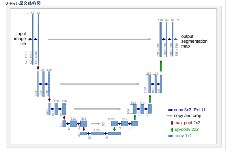
在图中可以看到下采样模块的每一块都有三层卷积,上采样也是如此,注意力机制是加在中间的那一层的,可以每一个模块都加,也可以加在其中的高层,但是这个模型对我的个人设备而言,参数量太大了,于是我没有采用那么大的层数,而且原始注意力模块是对图片进行patch分割,然后再进行注意力机制,而扩散模型中不用做patch,直接将输入reshape成B,H\*W,C,做注意力,然后再reshape成B,C,H,W。
对于我的实现,我加入了多头注意力机制之后的效果反而变得十分的差,应该是我加入的位置和方式不对,导致注意力没有起到正的作用。
对于模型的训练损失,损失会越来越低,而且第一步的损失就已经是在1以下很多,与平常很多模型训练得到的损失很不一样,可能是采样到的时间步t很小,噪声尺度也很小,MSE得到的本身就是个很小的数值
M S E = 1 N ∑ i ( ϵ ^ i − ϵ i ) 2 MSE = \frac{1}{N}\sum_i(\hat{\epsilon}_i - \epsilon_i)^2 MSE=N1∑i(ϵ^i−ϵi)2
真实值 ϵ i = 0.01 \epsilon_i=0.01 ϵi=0.01很小,即使预测的完全不正确,假设预测到 ϵ ^ i = 0.99 \hat{\epsilon}_i=0.99 ϵ^i=0.99,那么经过计算 ∑ i ( ϵ ^ i − ϵ i ) 2 = 0.9604 \sum_i(\hat{\epsilon}_i - \epsilon_i)^2=0.9604 ∑i(ϵ^i−ϵi)2=0.9604除以N之后就会更加的小,即使预测完全错误,均方误差的值也没有很大,所以误差并不能反应模型是不是收敛了,解决办法是根据不同的时间步进行检测,计算每中不同的时间步(比如0-100、100-200...)的损失是不是在下降。
2 RCNN
同时还在实现RCNN部分的代码,但是遇到了一些问题:
- 图片的尺寸大小不一致,每一张图片中的类的数量也不一致,导致读取得到的batch内的数据不等长;
- 可以借助opencv-python的selective search算法实现,但是算法的依赖和torch-cuda的依赖冲突;
尝试自己实现selective search算法来解决依赖冲突,但是实现上有难度。
总结
本周对之前的扩散模型进行重新的学习,弄清楚之前的不理解的点,并且通过代码实现了解了工作的基本流程。在完成了diffusion model之后还对rcnn进行了尝试,但是还没有解决相关的问题。