Contents
- [The Bitter Lesson: Scale!](#The Bitter Lesson: Scale!)
- [Self-Attention in Encoder: Dot-Product Attention](#Self-Attention in Encoder: Dot-Product Attention)
- [Masked-Attention in Decoder: Auto-Regressive Nature](#Masked-Attention in Decoder: Auto-Regressive Nature)
- [Encoder-Decoder Attention / Cross Attention](#Encoder-Decoder Attention / Cross Attention)
- [Multi-Head Attention](#Multi-Head Attention)
- Reference
The Bitter Lesson: Scale!
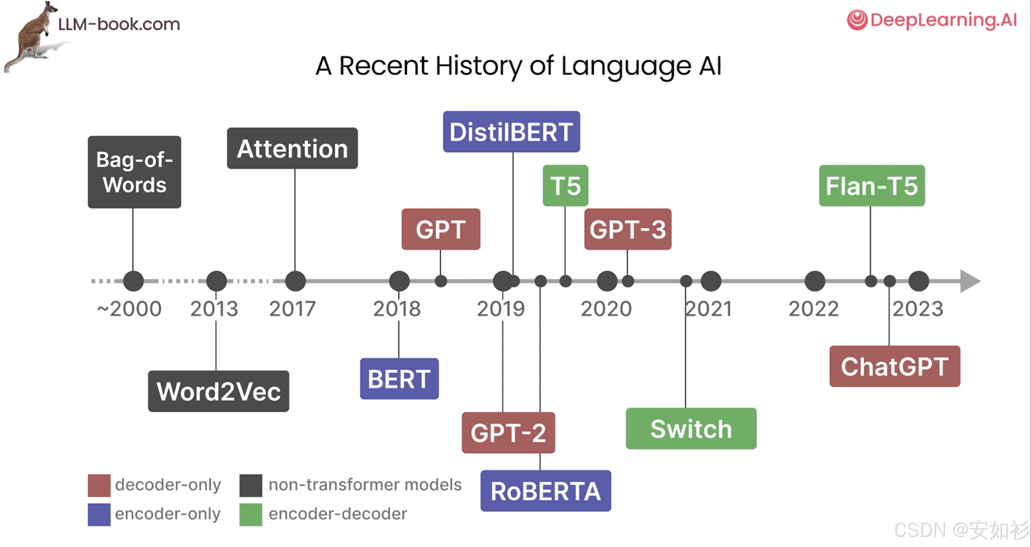
大型语言模型(LLM)的发展并非一蹴而就。其思想源头可追溯至1966年的聊天机器人ELIZA,而1997年长短期记忆(LSTM)网络的诞生,则为模型处理序列数据和学习文本规律奠定了基础。不过,RNN 一个显著缺点是无法无法在时间步上并行(当前时刻依赖上一个时刻)。
These researchers wanted methods based on human input to win and were disappointed when they did not. One thing that should be learned from the bitter lesson is the great power of general purpose methods, of methods that continue to scale with increased computation even as the available computation becomes very great.
Rich Sutton, The Bitter Lesson, March 13, 2019
真正的范式革命发生在2017年,Google发表了里程碑式的论文《Attention Is All You Need》,其中提出的Transformer架构完全摒弃了传统的 RNN 结构,仅依靠注意力机制(Attention Mechanism)并行处理数据,极大地提升了训练效率和性能。
这一突破开启了预训练模型的黄金时代。此后,各大科技巨头纷纷基于Transformer架构进行创新:Google 于2018年推出了里程碑式的BERT模型,其双向编码器结构在自然语言理解任务上表现卓越;OpenAI 则选择了 仅解码器(Decoder-only) 的路线,于2018年发布GPT-1,并在此基础上不断迭代。
随着模型规模的爆炸式增长,LLM的能力也实现了质的飞跃。2019年的GPT-2和2020年拥有1750亿参数的GPT-3,展示了惊人的少样本学习能力。 Google也推出了更大规模的PaLM模型,而Meta则通过发布LLaMA等模型,极大地促进了开源社区的繁荣。
2022年末,OpenAI发布的ChatGPT 引爆了全球范围内的AI热潮。 进入2023年,行业竞争愈发激烈,呈现出百花齐放的态势:OpenAI推出了更强大的多模态模型GPT-4,Google发布了Bard(后更名为Gemini)作为应对,Anthropic也推出了以安全为核心的Claude系列模型。2024至2025年,LLM的发展重心开始转向提升模型的深度推理能力,LLM正在从文字生成工具向具备更强推理与行动能力的智能体(Agent)方向加速演进。
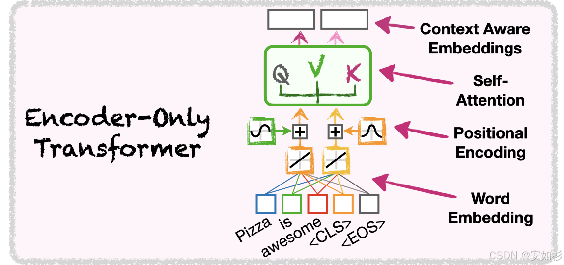
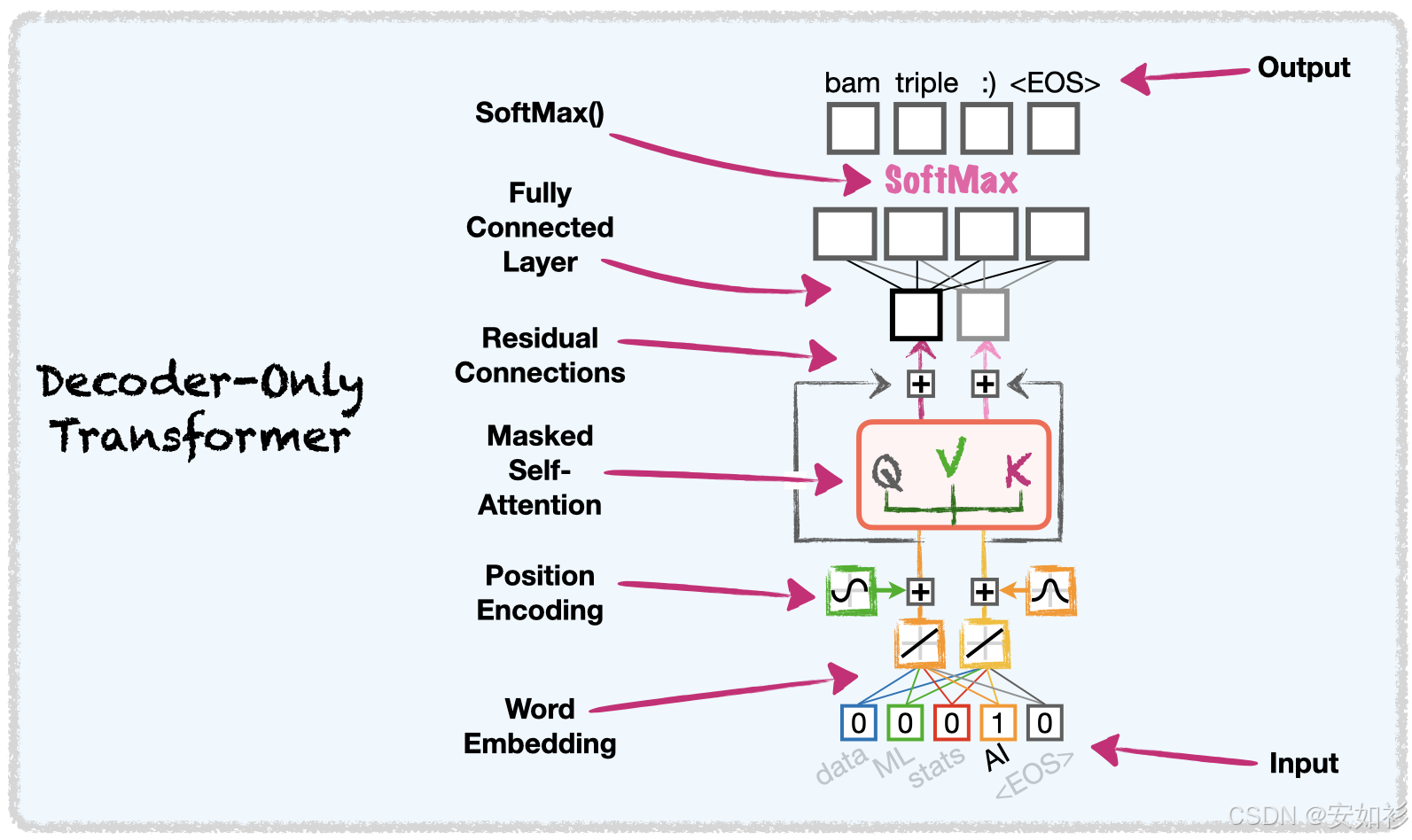
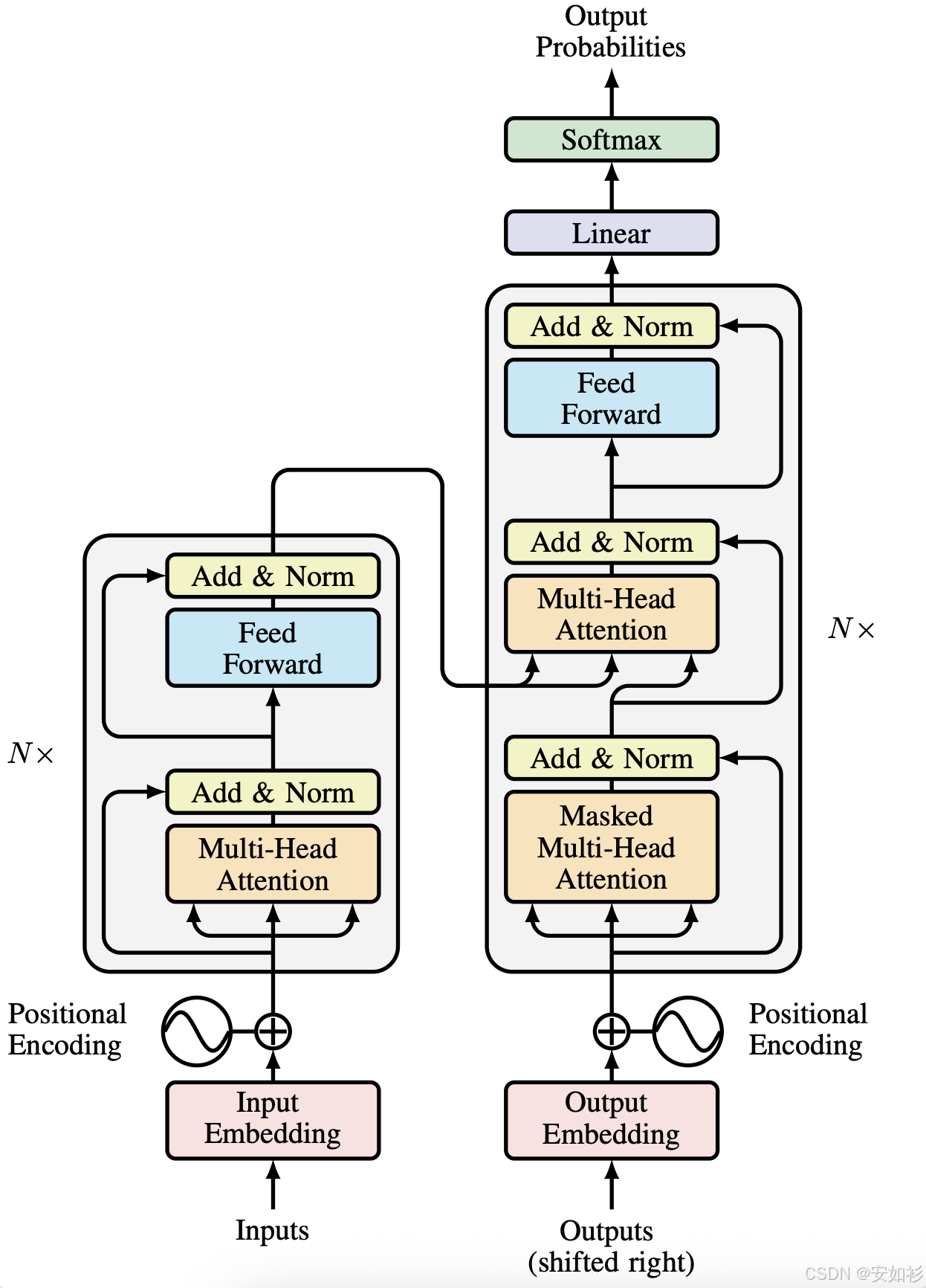
原始 Transformer 架构采用 Encoder-Decoder 架构,Encoder 负责整合上下文,Decoder 用于根据上下文做文字接龙。
- Encoder 可以用 RNN, CNN, Self-Attention ... 在原始 Transformer 架构中,采用 self-attention + residual + layer norm + FFN + residual + layer-norm 的 block。
- Decoder 一般是 Auto-Regressive 的方式,需要 Masked Self-Attention。
- Cross-Attention是Encoder-Decoder之间的桥梁,Encoder负责KV,Q来自于Decoder。
Transformer 三大核心组件&动机:
- 词必须表示为数字,否则没办法计算相似度,因此要有 Embedding Table/LM Head;
- 单词排列顺序也很重要,因此有 Positional Encoding;
- 词是带上下文的,词与词之间的关联性很重要,尤其是代词、多义词,因此有「注意力机制」。
Self-Attention in Encoder: Dot-Product Attention
- Attention 机制最早由 Bahdanau 等人在 2014 年提出,用于机器翻译任务中的 RNN 模型 。早期的 Attention 是 加性 机制,旨在让解码器在生成每个词时,能够"回头看"编码器的所有隐藏状态,并计算一个加权平均值作为上下文向量。
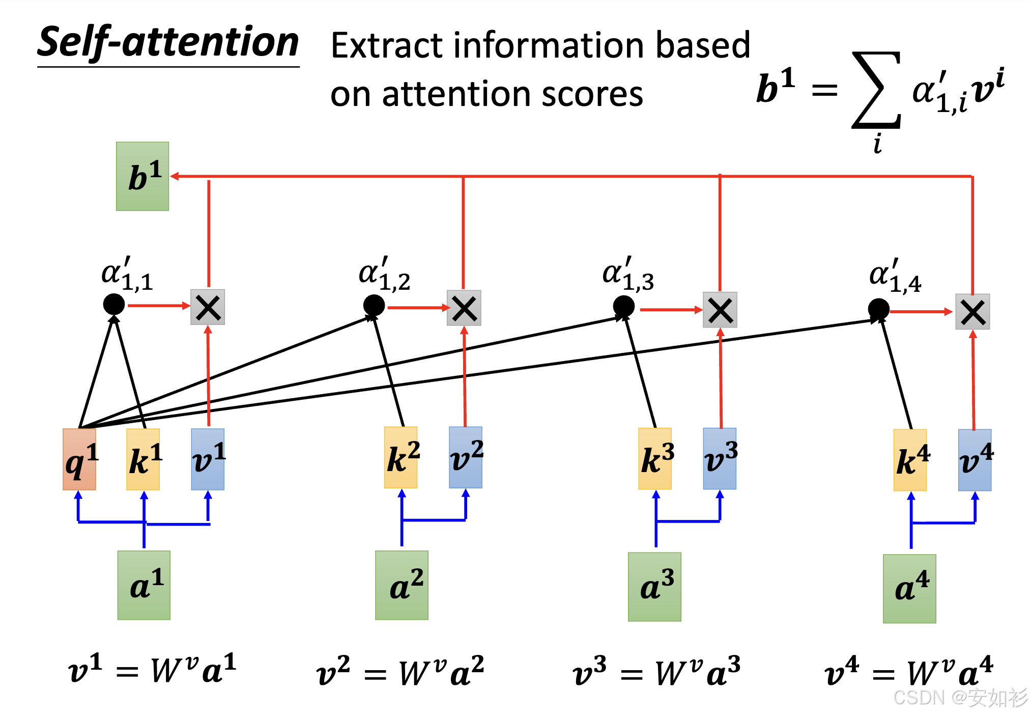
- 而"自注意力"(Self-Attention)是 乘性 机制,即序列中的每个元素都直接与序列中的其他所有元素进行交互,从而捕获全局依赖关系 ,因此复杂度为 O ( n 2 ) O(n^2) O(n2)。

核心步骤:
- 相关性计算:对于每个token都赋予(包括自己在内)所有token和当前token的"相关性"(反映语义距离),也就是计算 Q K T Q K^T QKT。为了减少 Softmax 饱和,从而保持梯度稳定, Q K T d k \frac{QK^T}{\sqrt{d_k}} dk QKT;为将分数转换为总和为 1 的权重值,添加 Softmax 非线性单元。
- 线性组合:根据权重,对 V V V进行加权求和,得到 Contextualized Embedding。
Query, Key, Value 是数据库术语,传统编程是 dictkey,硬查找要么找到要么没找到,然而 Soft Attention 是根据相似度加权提取所有可能的值,因为是连续的,所以可以通过梯度下降来训练,可以被认为是一种软查找表。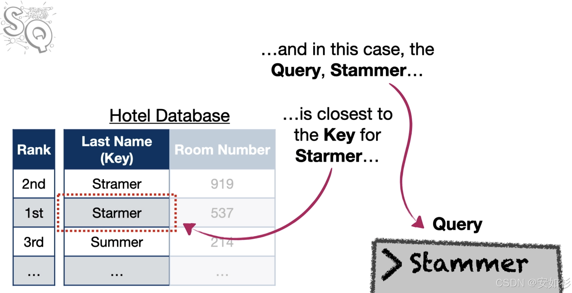
- 为什么不直接用 Embeddding 计算相似度,要对于每一个词都需要 Q/K 投影矩阵呢?
- 对称性限制(Symmetry Limitation):点积运算具有交换律,这意味着如果直接使用 X X X(Q=K=X),那么 Token A 对 Token B 的关注度将严格等于 Token B 对 Token A 的关注度。然而,语言中的关系往往是非对称的。例如,在句子"The animal didn't cross the street because it was too tired"中,代词"it"需要强烈关注"animal"以消除歧义,但"animal"本身并不需要同等程度地关注"it"来定义自身的语义。通过引入独立的 W Q W^Q WQ 和 W K W^K WK 线性变换,模型打破了这种对称性。
- 语义空间的解耦(Semantic Decoupling):同一个词在作为"查询者"和"被查询者"时,所代表的语义特征是不同的。 Q Q Q 向量代表"我在寻找什么特征", K K K 向量代表"我拥有什么特征"。线性投影将同一个词映射到了两个不同的功能子空间中。例如,动词可能会寻找(Query)对应的主语,而名词会展示(Key)其作为主语的属性。
- 为什么还需要 V 投影矩阵?
- 如果不使用 W V W^V WV(即 V = X V=X V=X),那么 Attention 层输出的仅仅是输入向量 X X X 的线性加权平均。输出永远处于输入向量构成的凸包(Convex Hull)内部。引入 W V W^V WV 后,不仅进行了加权平均,还对这些特征进行了线性变换(旋转、缩放)。这赋予了模型更强的表达能力,使其不仅仅是在"混合"原始词向量,而是在"混合"经过变换后的抽象特征。
- 信息过滤与特征提取:输入向量 X X X 同时包含了这个词的所有信息:词义、词性、时态、情感倾向、位置信息等。但是在某一个特定的注意力头(Head)中,并不需要传输所有的信息。如果令 V = X V=X V=X,那么无论 Attention 权重怎么变,传输的都是包含大量冗余噪音的原始向量 X X X,这会增加后续层处理信息的难度。假设我们在处理"I liked the movie"这句话。
- Head 1 的任务:关注时态(Grammar)。它计算出"liked"应该关注"I"(主谓一致)。此时,传递过去的 Value 应该主要是"过去时"这个特征,而不需要包含"喜欢"这个情感含义。
- Head 2 的任务:关注情感(Sentiment)。它计算出"liked"是情感核心。此时,传递过去的 Value 应该主要是"正面情感"这个特征,而不需要包含"动词"这个语法特征。
- Self-Attention 和 CNN 在特征提取上有什么不同?
- CNN 可以被解读成一种受限的 / 截断的 self-attention,因为 CNN 只考虑感受野(尺寸是超参数)内的资讯;Self-Attention 作为复杂版的 CNN,弹性更大,在训练资料少的时候容易"过拟合"(训练损失低,验证损失高)。RNN 和 Self- Attention 都是输入一个序列输出一个序列。
用于示例的代码:
python
class SelfAttention(nn.Module):

    def __init__(self, d_model=2,
                 row_dim=0,
                 col_dim=1):
        ## d_model = the number of embedding values per token.
        ##           Because we want to be able to do the math by hand, we've
        ##           the default value for d_model=2.
        ##           However, in "Attention Is All You Need" d_model=512
        ##
        ## row_dim, col_dim = the indices we should use to access rows or columns


        super().__init__()

        ## Initialize the Weights (W) that we'll use to create the
        ## query (q), key (k) and value (v) for each token
        ## NOTE: A lot of implementations include bias terms when
        ##       creating the the queries, keys, and values, but
        ##       the original manuscript that described Attention,
        ##       "Attention Is All You Need" did not, so we won't either
        self.W_q = nn.Linear(in_features=d_model, out_features=d_model, bias=False)
        self.W_k = nn.Linear(in_features=d_model, out_features=d_model, bias=False)
        self.W_v = nn.Linear(in_features=d_model, out_features=d_model, bias=False)

        self.row_dim = row_dim
        self.col_dim = col_dim


    def forward(self, token_encodings):
        ## Create the query, key and values using the encoding numbers
        ## associated with each token (token encodings)
        q = self.W_q(token_encodings)
        k = self.W_k(token_encodings)
        v = self.W_v(token_encodings)

        ## Compute similarities scores: (q * k^T)
        sims = torch.matmul(q, k.transpose(dim0=self.row_dim, dim1=self.col_dim))

        ## Scale the similarities by dividing by sqrt(k.col_dim)
        scaled_sims = sims / torch.tensor(k.size(self.col_dim)**0.5)

        ## Apply softmax to determine what percent of each tokens' value to
        ## use in the final attention values.
        attention_percents = F.softmax(scaled_sims, dim=self.col_dim)

        ## Scale the values by their associated percentages and add them up.
        attention_scores = torch.matmul(attention_percents, v)

        return attention_scores
Masked-Attention in Decoder: Auto-Regressive Nature
在 GPT 等解码器(Decoder-only)模型中,QKV 的计算受到 因果掩码(Causal Mask) 的限制。在预测下一个词时,模型不能"看到"未来的词。因此,在计算 Q K T QK^T QKT 后,我们将矩阵的上三角区域(代表未来位置)设为负无穷( − ∞ -\infty −∞)。结果:经过 Softmax 后,这些位置的概率变为 0。这意味着: Q t Q_t Qt(第 t 个时刻的查询)只能与 K 1 , . . . , K t K_1,..., K_t K1,...,Kt(当前及过去的键)进行交互,而不能与 K t + 1 K_{t+1} Kt+1 交互。这保证了生成的自回归性质。
用于示例的代码:
python
class MaskedSelfAttention(nn.Module):
    # ...
    def forward(self, token_encodings, mask=None):
	    # ...
        if mask is not None:
            ## Here we are masking out things we don't want to pay attention to
            ##
            ## We replace values we wanted masked out
            ## with a very small negative number so that the SoftMax() function
            ## will give all masked elements an output value (or "probability") of 0.
            scaled_sims = scaled_sims.masked_fill(mask=mask, value=-1e9) # I've also seen -1e20 and -9e15 used in masking
        # ...
        return attention_scores

## create the mask so that we don't use
## tokens that come after a token of interest
mask = torch.tril(torch.ones(3, 3))
mask = mask == 0
mask # print out the mask

## calculate masked self-attention
maskedSelfAttention(encodings_matrix, mask)
Encoder-Decoder Attention / Cross Attention
交叉注意力(Cross-Attention):连接编码器与解码器,Query 来自解码器(Decoder)的上一层输出,Key 和 Value 来自编码器(Encoder)的最终输出。
用于示例的代码:
python
class Attention(nn.Module):

    # ...

    ## The only change from SelfAttention and attention is that
    ## now we expect 3 sets of encodings to be passed in...
    def forward(self, encodings_for_q, encodings_for_k, encodings_for_v, mask=None):
        ## ...and we pass those sets of encodings to the various weight matrices.
        q = self.W_q(encodings_for_q)
        k = self.W_k(encodings_for_k)
        v = self.W_v(encodings_for_v)

        # ...
Multi-Head Attention
理解了单头注意力后,我们探讨 QKV 在更复杂场景下的行为。 MultiHead ( Q , K , V ) = Concat ( head 1 , . . . , head h ) W O \text{MultiHead}(Q, K, V) = \text{Concat}(\text{head}_1,..., \text{head}_h)W^O MultiHead(Q,K,V)=Concat(head1,...,headh)WO其中 head i = Attention ( Q W i Q , K W i K , V W i V ) \text{head}_i = \text{Attention}(QW_i^Q, KW_i^K, VW_i^V) headi=Attention(QWiQ,KWiK,VWiV)。为什么需要多头?单一的注意力机制可能无法同时捕捉句子的多重含义。例如句子:"The apple falls because it is ripe."Token "it" 需要关注 "apple"(指代关系)。Token "it" 同时也处于 "because" 引导的因果从句中(逻辑关系)。Token "ripe" 需要关注 "apple"(修饰关系)。单个 Head 的 QKV 很难同时为"指代"、"逻辑"、"修饰"进行最优的权重分配。多头机制允许模型在不同的"通道"上并行学习这些关系。
用于示例的代码:
python
class MultiHeadAttention(nn.Module):

    def __init__(self,
                 d_model=2,
                 row_dim=0,
                 col_dim=1,
                 num_heads=1):

        super().__init__()

        ## create a bunch of attention heads
        self.heads = nn.ModuleList(
            [Attention(d_model, row_dim, col_dim)
             for _ in range(num_heads)]
        )

        self.col_dim = col_dim

    def forward(self,
                encodings_for_q,
                encodings_for_k,
                encodings_for_v):

        ## run the data through all of the attention heads
        return torch.cat([head(encodings_for_q,
                               encodings_for_k,
                               encodings_for_v)
                          for head in self.heads], dim=self.col_dim)