下降算法
- 求
,计算
- 代回
- 迭代
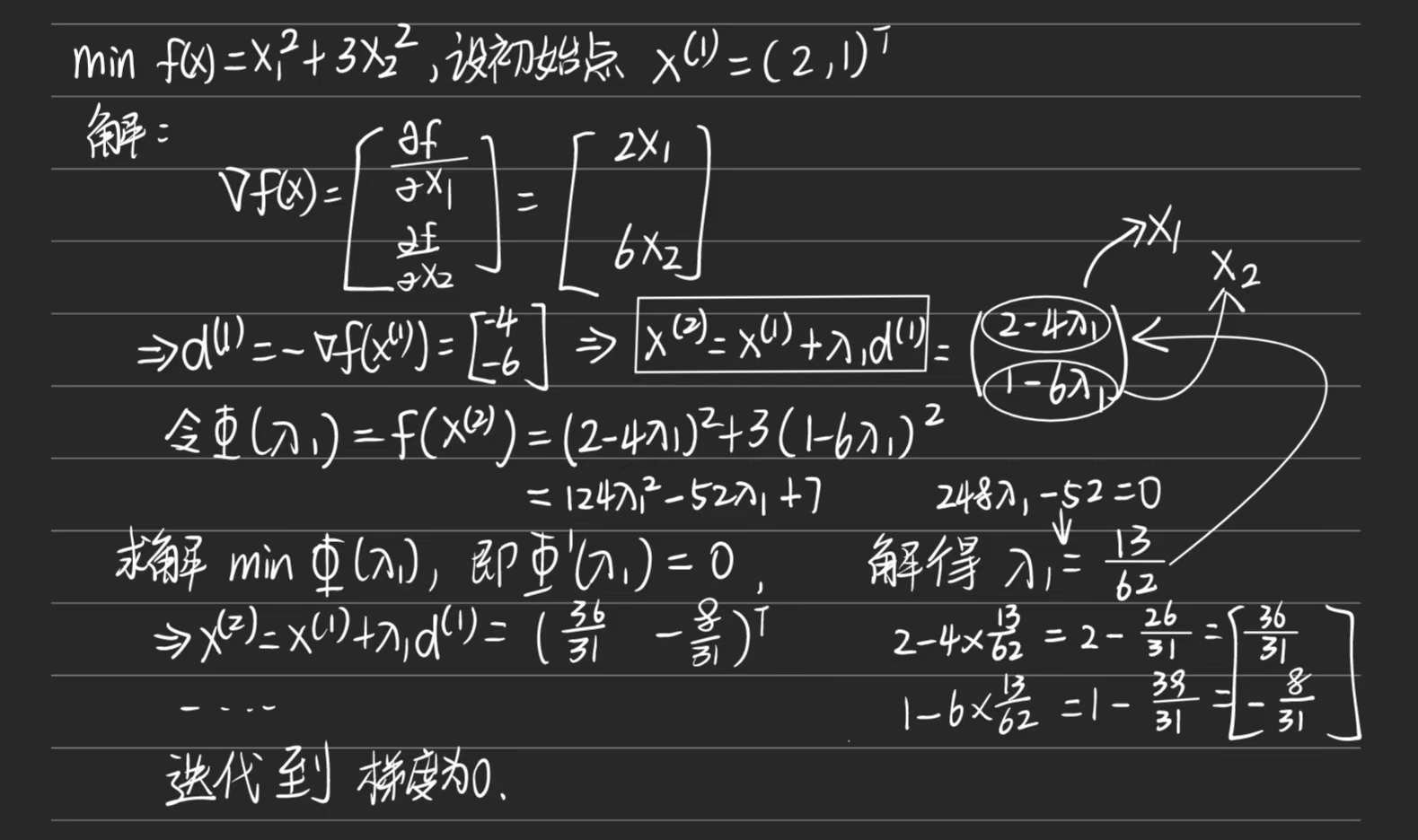
最速下降法(Steepest Descent Method)
-
原理:基于一阶导数(梯度),在每次迭代中,沿着当前点的负梯度方向(即函数值下降最快的方向)移动。步长通常通过线搜索(如精确线搜索或回溯线搜索)确定。
-
优点:实现简单,计算成本低,每步迭代只需计算梯度。
-
缺点:收敛速度慢(线性收敛),尤其在接近最小值时可能出现"锯齿"现象,即迭代路径振荡。
核心公式
-
梯度方向:
-
迭代公式:
-
步长选择(精确线搜索):
算法步骤
-
计算梯度
-
确定下降方向
-
线性搜索求步长
-
更新迭代点
例题
,设初始点
代码
封装函数的表达式。
python
def f(x):
    """目标函数:f(x) = x1^2 + 3*x2^2"""
    return x[0] ** 2 + 3 * x[1] ** 2
封装函数的梯度。
python
def gradient(x):
    """计算梯度:∇f(x) = [2*x1, 6*x2]"""
    return np.array([2 * x[0], 6 * x[1]])
设置初始点。
python
# 设置初始点
x0 = np.array([2.0, 1.0])
最速下降法核心算法。
python
def steepest_descent_improved(x0, max_iter=100, tol=1e-6, x_tol=1e-8):
    """
    改进的最速下降法,包含多重停止准则
    """
    x_history = [x0.copy()]  # 保存x的历史值
    f_history = [f(x0)]  # 保存函数值的历史
    grad_history = [gradient(x0)]  # 保存梯度的历史

    x = x0.copy()  # 当前点

    for i in range(max_iter):
        grad = gradient(x)  # 计算当前梯度
        grad_norm = np.linalg.norm(grad)  # 计算梯度范数

        # 检查多重收敛准则
        # 1. 梯度接近零
        if grad_norm < tol:
            print(f"通过梯度准则在 {i + 1} 次迭代后收敛")
            break

        # 2. x的变化可忽略
        if i > 0:
            x_change = np.linalg.norm(x_history[-1] - x_history[-2])
            if x_change < x_tol:
                print(f"通过x变化准则在 {i + 1} 次迭代后收敛")
                break

        # 3. 函数值变化可忽略
        if i > 0:
            f_change = abs(f_history[-1] - f_history[-2])
            if f_change < tol:
                print(f"通过函数值准则在 {i + 1} 次迭代后收敛")
                break

        # 精确线搜索计算步长
        alpha = exact_line_search(x, grad)

        # 更新点
        x_new = x - alpha * grad

        # 检查更新是否显著
        if np.linalg.norm(x_new - x) < 1e-15:
            print(f"更新可忽略,在 {i + 1} 次迭代后停止")
            break

        x = x_new

        # 保存历史记录
        x_history.append(x.copy())
        f_history.append(f(x))
        grad_history.append(grad.copy())

    return np.array(x_history), np.array(f_history), np.array(grad_history)
完整代码
python
import numpy as np
import matplotlib.pyplot as plt
def f(x):
"""目标函数:f(x) = x1^2 + 3*x2^2"""
return x[0] ** 2 + 3 * x[1] ** 2
def gradient(x):
"""计算梯度:grad f(x) = [2*x1, 6*x2]"""
return np.array([2 * x[0], 6 * x[1]])
def exact_line_search(x, grad):
"""精确线搜索计算最优步长"""
# 对于二次函数 f(x) = x1^2 + 3*x2^2
# 最小化 f(x - α∇f(x)) 关于α
# 解析解为 α = (∇f(x)^T ∇f(x)) / (∇f(x)^T H ∇f(x))
# 其中 H 是 Hessian 矩阵 [[2, 0], [0, 6]]
numerator = grad[0] ** 2 + grad[1] ** 2
denominator = 2 * grad[0] ** 2 + 6 * grad[1] ** 2
return numerator / denominator
def steepest_descent_improved(x0, max_iter=100, tol=1e-6, x_tol=1e-8):
"""
改进的最速下降法,包含多重停止准则
"""
x_history = [x0.copy()] # 保存x的历史值
f_history = [f(x0)] # 保存函数值的历史
grad_history = [gradient(x0)] # 保存梯度的历史
x = x0.copy() # 当前点
for i in range(max_iter):
grad = gradient(x) # 计算当前梯度
grad_norm = np.linalg.norm(grad) # 计算梯度范数
# 检查多重收敛准则
# 1. 梯度接近零
if grad_norm < tol:
print(f"通过梯度准则在 {i + 1} 次迭代后收敛")
break
# 2. x的变化可忽略
if i > 0:
x_change = np.linalg.norm(x_history[-1] - x_history[-2])
if x_change < x_tol:
print(f"通过x变化准则在 {i + 1} 次迭代后收敛")
break
# 3. 函数值变化可忽略
if i > 0:
f_change = abs(f_history[-1] - f_history[-2])
if f_change < tol:
print(f"通过函数值准则在 {i + 1} 次迭代后收敛")
break
# 精确线搜索计算步长
alpha = exact_line_search(x, grad)
# 更新点
x_new = x - alpha * grad
# 检查更新是否显著
if np.linalg.norm(x_new - x) < 1e-15:
print(f"更新可忽略,在 {i + 1} 次迭代后停止")
break
x = x_new
# 保存历史记录
x_history.append(x.copy())
f_history.append(f(x))
grad_history.append(grad.copy())
return np.array(x_history), np.array(f_history), np.array(grad_history)
# 设置初始点
x0 = np.array([2.0, 1.0])
x_history, f_history, grad_history = steepest_descent_improved(x0, max_iter=50, tol=1e-6, x_tol=1e-8)
# 打印结果
print("\n迭代历史:")
for i, (x, f_val, grad) in enumerate(zip(x_history, f_history, grad_history)):
grad_norm = np.linalg.norm(grad)
print(f"迭代 {i}: x = ({x[0]:.6f}, {x[1]:.6f}), f(x) = {f_val:.6f}, 梯度范数 = {grad_norm:.2e}")
print(f"\n最终结果: x = ({x_history[-1, 0]:.10f}, {x_history[-1, 1]:.10f}), f(x) = {f_history[-1]:.10f}")
# 绘制结果
plt.figure(figsize=(15, 5))
# 1. 等高线图和迭代路径
plt.subplot(1, 3, 1)
x1 = np.linspace(-0.5, 2.5, 100)
x2 = np.linspace(-1.0, 1.5, 100)
X1, X2 = np.meshgrid(x1, x2)
Z = X1 ** 2 + 3 * X2 ** 2
# 绘制等高线
contour = plt.contour(X1, X2, Z, levels=20, alpha=0.6)
plt.clabel(contour, inline=True, fontsize=8)
# 绘制迭代路径
plt.plot(x_history[:, 0], x_history[:, 1], 'ro-', markersize=4, linewidth=1, label='Iteration Path')
plt.plot(x0[0], x0[1], 'bs', markersize=8, label='Initial Point (2,1)')
plt.plot(0, 0, 'g*', markersize=10, label='Minimum Point (0,0)')
plt.xlabel('x1')
plt.ylabel('x2')
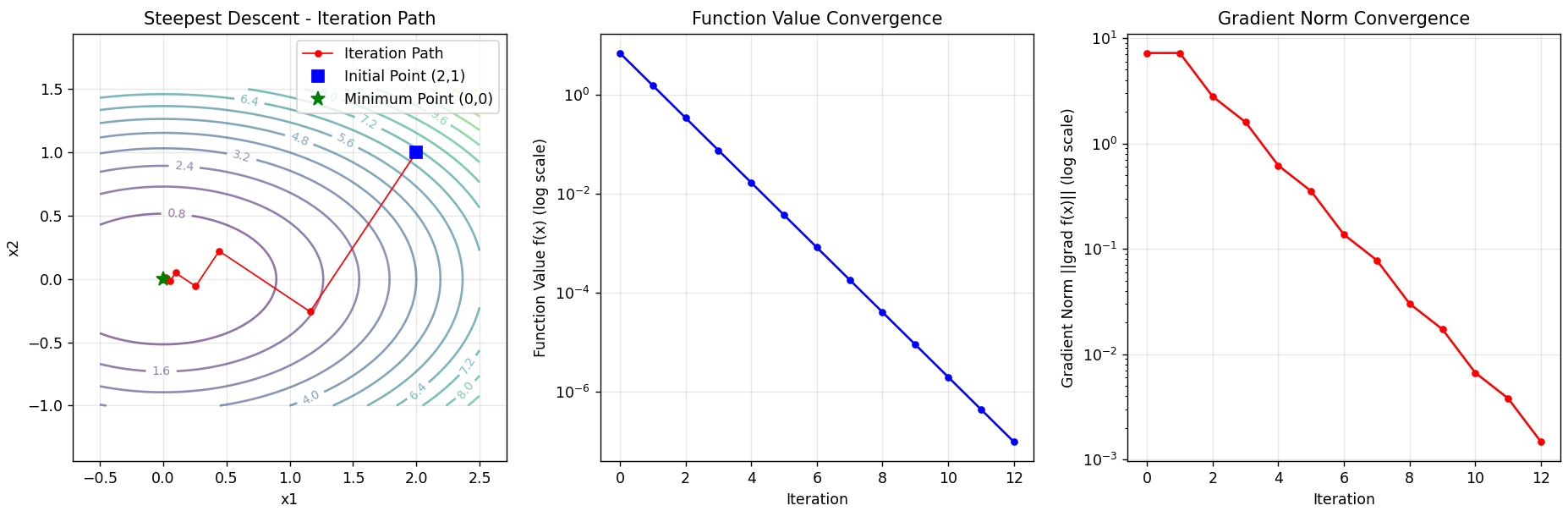
plt.title('Steepest Descent - Iteration Path')
plt.legend()
plt.grid(True, alpha=0.3)
plt.axis('equal')
# 2. 函数值收敛图
plt.subplot(1, 3, 2)
plt.semilogy(f_history, 'b-o', markersize=4)
plt.xlabel('Iteration')
plt.ylabel('Function Value f(x) (log scale)')
plt.title('Function Value Convergence')
plt.grid(True, alpha=0.3)
# 3. 梯度范数收敛图
plt.subplot(1, 3, 3)
grad_norms = [np.linalg.norm(grad) for grad in grad_history]
plt.semilogy(grad_norms, 'r-o', markersize=4)
plt.xlabel('Iteration')
plt.ylabel('Gradient Norm ||grad f(x)|| (log scale)')
plt.title('Gradient Norm Convergence')
plt.grid(True, alpha=0.3)
plt.tight_layout()
plt.show()=(1.16129,−0.258065).
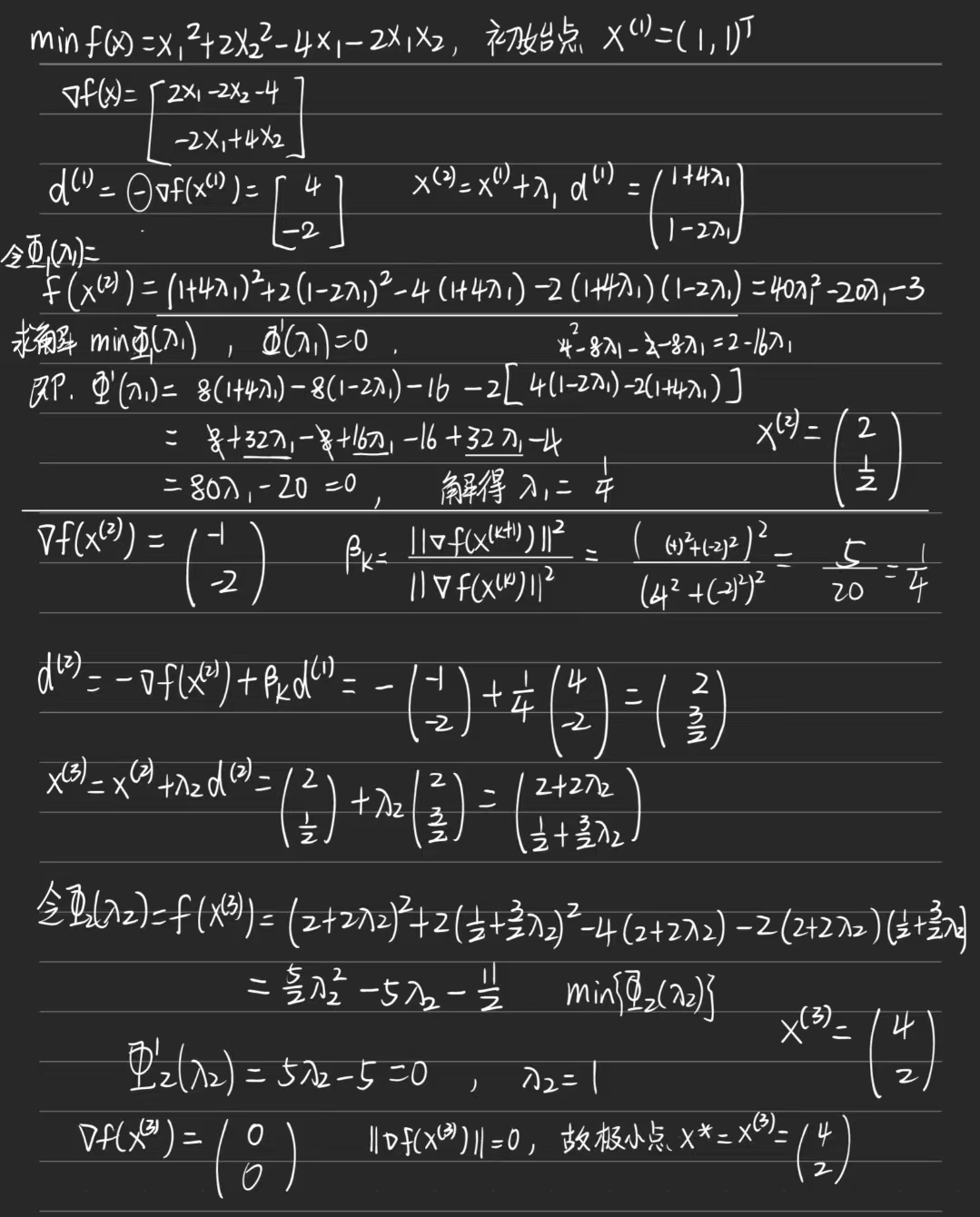
共轭梯度法(Conjugate Gradient Method)
-
原理:结合梯度信息和共轭方向,用于加速收敛。对于二次函数,它生成一组共轭方向,使得在每个方向上梯度正交,从而避免锯齿现象。对于一般函数,它使用梯度信息构建共轭方向。
-
优点:收敛速度比最速下降法快(超线性收敛),内存需求低,只需存储少量向量。
-
缺点:对于非二次函数,性能依赖于线搜索的精度;可能对初始点敏感。
核心公式
-
迭代公式:
-
共轭方向:
-
β系数(Fletcher-Reeves公式):
-
β系数(Polak-Ribière公式):
算法步骤
-
初始方向
-
线搜索求 αk
-
更新
-
计算新梯度
-
计算
例题
,初始点
代码
python
import numpy as np
import matplotlib.pyplot as plt


def f(x):
    """目标函数:f(x) = x₁² + 2x₂² - 4x₁ - 2x₁x₂"""
    return x[0] ** 2 + 2 * x[1] ** 2 - 4 * x[0] - 2 * x[0] * x[1]


def gradient(x):
    """计算梯度:∇f(x) = [2x₁ - 4 - 2x₂, 4x₂ - 2x₁]"""
    return np.array([2 * x[0] - 4 - 2 * x[1], 4 * x[1] - 2 * x[0]])


def exact_line_search(x, d):
    """
    精确线搜索确定步长
    通过最小化 φ(α) = f(x + αd) 关于α
    """
    # 将x + αd代入目标函数
    x1_new = x[0] + d[0]
    x2_new = x[1] + d[1]

    # 展开 f(x + αd) 得到关于α的二次函数
    # f(x + αd) = (x1 + αd1)² + 2(x2 + αd2)² - 4(x1 + αd1) - 2(x1 + αd1)(x2 + αd2)
    # 展开并整理得到 Aα² + Bα + C 的形式
    A = d[0] ** 2 + 2 * d[1] ** 2 - 2 * d[0] * d[1]
    B = 2 * x[0] * d[0] + 4 * x[1] * d[1] - 4 * d[0] - 2 * x[0] * d[1] - 2 * x[1] * d[0]
    C = x[0] ** 2 + 2 * x[1] ** 2 - 4 * x[0] - 2 * x[0] * x[1]

    # 二次函数的最小值在 α = -B/(2A)
    if A != 0:
        alpha = -B / (2 * A)
    else:
        alpha = 0  # 如果A=0,函数是线性的,无法通过此方法找到最小值

    return alpha


def conjugate_gradient(x0, max_iter=10, tol=1e-6):
    """
    共轭梯度法实现

    参数:
    x0: 初始点
    max_iter: 最大迭代次数
    tol: 收敛容差

    返回:
    x_history: 迭代点历史
    f_history: 函数值历史
    grad_history: 梯度历史
    """
    # 初始化
    x = x0.copy()
    g = gradient(x)  # 初始梯度
    d = -g  # 初始搜索方向

    # 保存历史记录
    x_history = [x.copy()]
    f_history = [f(x)]
    grad_history = [g.copy()]

    print("初始点:")
    print(f"x0 = ({x[0]}, {x[1]}), f(x0) = {f(x):.4f}, ∇f(x0) = ({g[0]}, {g[1]})")
    print(f"初始搜索方向 d0 = ({d[0]}, {d[1]})")
    print()

    for k in range(max_iter):
        print(f"=== 第 {k + 1} 次迭代 ===")

        # 1. 线搜索确定步长
        alpha = exact_line_search(x, d)
        print(f"步长 α_{k} = {alpha:.4f}")

        # 2. 更新点
        x_new = x + alpha * d
        print(
            f"更新点: x_{k + 1} = x_{k} + α_{k} * d_{k} = ({x[0]:.4f}, {x[1]:.4f}) + {alpha:.4f} * ({d[0]:.4f}, {d[1]:.4f}) = ({x_new[0]:.4f}, {x_new[1]:.4f})")

        # 3. 计算新梯度
        g_new = gradient(x_new)
        print(f"新梯度: ∇f(x_{k + 1}) = ({g_new[0]:.4f}, {g_new[1]:.4f})")

        # 检查收敛
        grad_norm = np.linalg.norm(g_new)
        if grad_norm < tol:
            print(f"\n梯度范数 {grad_norm:.6f} < 容差 {tol},算法收敛!")
            break

        # 4. 计算共轭参数 (Fletcher-Reeves公式)
        beta = np.dot(g_new, g_new) / np.dot(g, g)
        print(
            f"共轭参数 β_{k} = (g_{k + 1}·g_{k + 1}) / (g_{k}·g_{k}) = {np.dot(g_new, g_new):.4f} / {np.dot(g, g):.4f} = {beta:.4f}")

        # 5. 更新搜索方向
        d_new = -g_new + beta * d
        print(
            f"新搜索方向: d_{k + 1} = -g_{k + 1} + β_{k} * d_{k} = -({g_new[0]:.4f}, {g_new[1]:.4f}) + {beta:.4f} * ({d[0]:.4f}, {d[1]:.4f}) = ({d_new[0]:.4f}, {d_new[1]:.4f})")

        # 保存历史记录
        x_history.append(x_new.copy())
        f_history.append(f(x_new))
        grad_history.append(g_new.copy())

        # 为下一次迭代更新变量
        x = x_new
        g = g_new
        d = d_new

        print()

    return np.array(x_history), np.array(f_history), np.array(grad_history)


def visualize_results(x_history, f_history, grad_history):
    """可视化结果"""
    # 创建等高线图
    plt.figure(figsize=(15, 5))

    # 1. 等高线图和迭代路径
    plt.subplot(1, 3, 1)
    x1 = np.linspace(0, 5, 100)
    x2 = np.linspace(0, 3, 100)
    X1, X2 = np.meshgrid(x1, x2)
    Z = X1 ** 2 + 2 * X2 ** 2 - 4 * X1 - 2 * X1 * X2

    # 绘制等高线
    contour = plt.contour(X1, X2, Z, levels=20, alpha=0.6)
    plt.clabel(contour, inline=True, fontsize=8)

    # 绘制迭代路径
    plt.plot(x_history[:, 0], x_history[:, 1], 'ro-', markersize=6, linewidth=2, label='Iteration Path')
    plt.plot(x_history[0, 0], x_history[0, 1], 'bs', markersize=10, label='Initial Point (1,1)')
    plt.plot(x_history[-1, 0], x_history[-1, 1], 'g*', markersize=15,
             label=f'Final Point ({x_history[-1, 0]:.2f},{x_history[-1, 1]:.2f})')

    # 标记最优解
    plt.plot(4, 2, 'md', markersize=10, label='Optimal Point (4,2)')

    plt.xlabel('x1')
    plt.ylabel('x2')
    plt.title('Conjugate Gradient - Iteration Path')
    plt.legend()
    plt.grid(True, alpha=0.3)
    plt.axis('equal')

    # 2. 函数值收敛图
    plt.subplot(1, 3, 2)
    plt.plot(f_history, 'b-o', markersize=6, linewidth=2)
    plt.xlabel('Iteration')
    plt.ylabel('Function Value f(x)')
    plt.title('Function Value Convergence')
    plt.grid(True, alpha=0.3)

    # 3. 梯度范数收敛图
    plt.subplot(1, 3, 3)
    grad_norms = [np.linalg.norm(grad) for grad in grad_history]
    plt.semilogy(grad_norms, 'r-o', markersize=6, linewidth=2)
    plt.xlabel('Iteration')
    plt.ylabel('Gradient Norm ||∇f(x)|| (log scale)')
    plt.title('Gradient Norm Convergence')
    plt.grid(True, alpha=0.3)

    plt.tight_layout()
    plt.show()


def analytical_solution():
    """计算解析解"""
    print("\n=== 解析解验证 ===")
    # 解方程组: ∇f(x) = 0
    # 2x₁ - 4 - 2x₂ = 0
    # 4x₂ - 2x₁ = 0

    # 从第二个方程: 4x₂ = 2x₁ => x₂ = x₁/2
    # 代入第一个方程: 2x₁ - 4 - 2(x₁/2) = 0 => 2x₁ - 4 - x₁ = 0 => x₁ = 4
    # 然后 x₂ = 4/2 = 2

    x_opt = np.array([4.0, 2.0])
    f_opt = f(x_opt)

    print(f"通过解方程组 ∇f(x) = 0 得到:")
    print("2x₁ - 4 - 2x₂ = 0")
    print("4x₂ - 2x₁ = 0")
    print(f"解得: x₁ = 4, x₂ = 2")
    print(f"最优解: x* = ({x_opt[0]}, {x_opt[1]})")
    print(f"最优值: f(x*) = {f_opt:.6f}")

    return x_opt, f_opt


# 主程序
if __name__ == "__main__":
    # 设置初始点
    x0 = np.array([1.0, 1.0])

    # 运行共轭梯度法
    print("开始共轭梯度法求解...")
    print("目标函数: f(x) = x₁² + 2x₂² - 4x₁ - 2x₁x₂")
    print(f"初始点: x⁽¹⁾ = ({x0[0]}, {x0[1]})")
    print()

    x_history, f_history, grad_history = conjugate_gradient(x0, max_iter=10, tol=1e-6)

    # 打印最终结果
    print("\n=== 最终结果 ===")
    print(f"最优解: x* = ({x_history[-1, 0]:.6f}, {x_history[-1, 1]:.6f})")
    print(f"最优值: f(x*) = {f_history[-1]:.6f}")
    print(f"梯度范数: ||∇f(x*)|| = {np.linalg.norm(grad_history[-1]):.2e}")
    print(f"迭代次数: {len(x_history) - 1}")

    # 计算解析解
    x_opt, f_opt = analytical_solution()

    # 计算误差
    error_x = np.linalg.norm(x_history[-1] - x_opt)
    error_f = abs(f_history[-1] - f_opt)

    print(f"\n=== 误差分析 ===")
    print(f"解向量误差: ||x_cg - x_opt|| = {error_x:.2e}")
    print(f"函数值误差: |f_cg - f_opt| = {error_f:.2e}")

    # 可视化结果
    visualize_results(x_history, f_history, grad_history)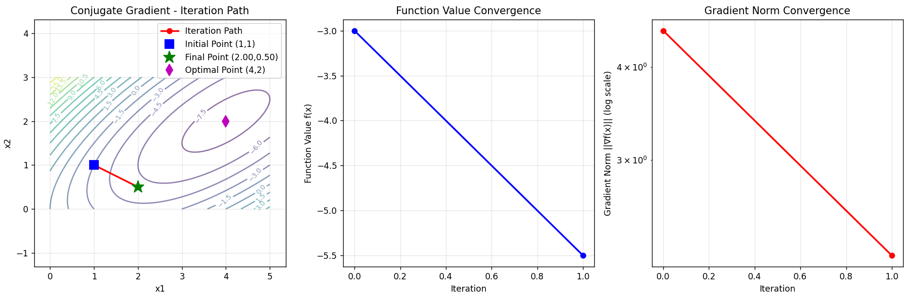
牛顿法(Newton's Method)
-
原理:利用二阶导数(Hessian矩阵)信息,通过求解牛顿方程(Hessian矩阵的逆乘以梯度)得到下降方向。步长通常设为1,但可能需调整。
-
优点:收敛速度快(二次收敛),如果初始点接近最小值,效率很高。
-
缺点:需要计算和存储Hessian矩阵及其逆,计算成本高;Hessian矩阵可能非正定,导致算法失败。
核心公式
-
牛顿方程:
-
迭代公式:
-
或显式写出:
算法步骤
-
计算梯度
-
计算Hessian矩阵
-
解线性方程组
-
更新
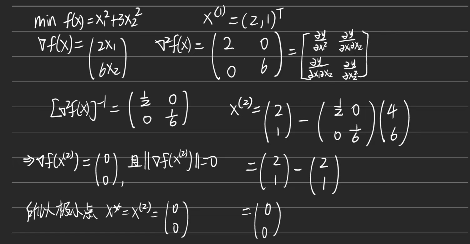
例题
,
代码
python
import numpy as np
import matplotlib.pyplot as plt


def f(x):
    """目标函数:f(x) = x₁² + 3x₂²"""
    return x[0] ** 2 + 3 * x[1] ** 2


def gradient(x):
    """计算梯度:∇f(x) = [2x₁, 6x₂]"""
    return np.array([2 * x[0], 6 * x[1]])


def hessian(x):
    """计算Hessian矩阵:H = [[2, 0], [0, 6]] (常数矩阵)"""
    # 对于二次函数,Hessian矩阵是常数
    return np.array([[2, 0], [0, 6]])


def newton_method(x0, max_iter=10, tol=1e-6):
    """
    牛顿法实现

    参数:
    x0: 初始点
    max_iter: 最大迭代次数
    tol: 收敛容差

    返回:
    x_history: 迭代点历史
    f_history: 函数值历史
    grad_history: 梯度历史
    """
    # 初始化
    x = x0.copy()

    # 保存历史记录
    x_history = [x.copy()]
    f_history = [f(x)]
    grad_history = [gradient(x)]

    print("初始点:")
    print(f"x0 = ({x[0]}, {x[1]}), f(x0) = {f(x):.4f}, ∇f(x0) = ({grad_history[0][0]}, {grad_history[0][1]})")
    print()

    for k in range(max_iter):
        print(f"=== 第 {k + 1} 次迭代 ===")

        # 计算当前梯度和Hessian矩阵
        g = gradient(x)
        H = hessian(x)

        print(f"梯度: ∇f(x_{k}) = ({g[0]:.4f}, {g[1]:.4f})")
        print(f"Hessian矩阵: H = [[{H[0, 0]}, {H[0, 1]}], [{H[1, 0]}, {H[1, 1]}]]")

        # 检查Hessian矩阵是否正定
        eigenvalues = np.linalg.eigvals(H)
        if np.all(eigenvalues > 0):
            print(f"Hessian矩阵特征值: {eigenvalues} (正定)")
        else:
            print(f"Hessian矩阵特征值: {eigenvalues} (非正定)")

        # 计算牛顿方向: d = -H^{-1} * g
        try:
            H_inv = np.linalg.inv(H)
            d = -H_inv @ g
            print(f"牛顿方向: d_{k} = -H⁻¹ * ∇f(x_{k}) = ({d[0]:.4f}, {d[1]:.4f})")
        except np.linalg.LinAlgError:
            print("Hessian矩阵奇异,无法求逆")
            break

        # 更新点: x_{k+1} = x_k + d_k
        x_new = x + d
        print(
            f"更新点: x_{k + 1} = x_{k} + d_{k} = ({x[0]:.4f}, {x[1]:.4f}) + ({d[0]:.4f}, {d[1]:.4f}) = ({x_new[0]:.4f}, {x_new[1]:.4f})")

        # 计算新梯度
        g_new = gradient(x_new)
        print(f"新梯度: ∇f(x_{k + 1}) = ({g_new[0]:.4f}, {g_new[1]:.4f})")

        # 保存历史记录
        x_history.append(x_new.copy())
        f_history.append(f(x_new))
        grad_history.append(g_new.copy())

        # 检查收敛
        grad_norm = np.linalg.norm(g_new)
        if grad_norm < tol:
            print(f"\n梯度范数 {grad_norm:.6f} < 容差 {tol},算法收敛!")
            break

        # 为下一次迭代更新变量
        x = x_new

        print()

    return np.array(x_history), np.array(f_history), np.array(grad_history)


def visualize_results(x_history, f_history, grad_history):
    """可视化结果"""
    # 创建等高线图
    plt.figure(figsize=(15, 5))

    # 1. 等高线图和迭代路径
    plt.subplot(1, 3, 1)
    x1 = np.linspace(-0.5, 2.5, 100)
    x2 = np.linspace(-0.5, 1.5, 100)
    X1, X2 = np.meshgrid(x1, x2)
    Z = X1 ** 2 + 3 * X2 ** 2

    # 绘制等高线
    contour = plt.contour(X1, X2, Z, levels=20, alpha=0.6)
    plt.clabel(contour, inline=True, fontsize=8)

    # 绘制迭代路径
    plt.plot(x_history[:, 0], x_history[:, 1], 'ro-', markersize=6, linewidth=2, label='Iteration Path')
    plt.plot(x_history[0, 0], x_history[0, 1], 'bs', markersize=10, label='Initial Point (2,1)')
    plt.plot(x_history[-1, 0], x_history[-1, 1], 'g*', markersize=15,
             label=f'Final Point ({x_history[-1, 0]:.2f},{x_history[-1, 1]:.2f})')

    # 标记最优解
    plt.plot(0, 0, 'md', markersize=10, label='Optimal Point (0,0)')

    plt.xlabel('x1')
    plt.ylabel('x2')
    plt.title('Newton Method - Iteration Path')
    plt.legend()
    plt.grid(True, alpha=0.3)
    plt.axis('equal')

    # 2. 函数值收敛图
    plt.subplot(1, 3, 2)
    plt.plot(f_history, 'b-o', markersize=6, linewidth=2)
    plt.xlabel('Iteration')
    plt.ylabel('Function Value f(x)')
    plt.title('Function Value Convergence')
    plt.grid(True, alpha=0.3)

    # 3. 梯度范数收敛图
    plt.subplot(1, 3, 3)
    grad_norms = [np.linalg.norm(grad) for grad in grad_history]
    plt.semilogy(grad_norms, 'r-o', markersize=6, linewidth=2)
    plt.xlabel('Iteration')
    plt.ylabel('Gradient Norm ||∇f(x)|| (log scale)')
    plt.title('Gradient Norm Convergence')
    plt.grid(True, alpha=0.3)

    plt.tight_layout()
    plt.show()


def analytical_solution():
    """计算解析解"""
    print("\n=== 解析解验证 ===")
    # 解方程组: ∇f(x) = 0
    # 2x₁ = 0
    # 6x₂ = 0

    x_opt = np.array([0.0, 0.0])
    f_opt = f(x_opt)

    print(f"通过解方程组 ∇f(x) = 0 得到:")
    print("2x₁ = 0")
    print("6x₂ = 0")
    print(f"解得: x₁ = 0, x₂ = 0")
    print(f"最优解: x* = ({x_opt[0]}, {x_opt[1]})")
    print(f"最优值: f(x*) = {f_opt:.6f}")

    return x_opt, f_opt


# 主程序
if __name__ == "__main__":
    # 设置初始点
    x0 = np.array([2.0, 1.0])

    # 运行牛顿法
    print("开始牛顿法求解...")
    print("目标函数: f(x) = x₁² + 3x₂²")
    print(f"初始点: x⁽¹⁾ = ({x0[0]}, {x0[1]})")
    print()

    x_history, f_history, grad_history = newton_method(x0, max_iter=10, tol=1e-6)

    # 打印最终结果
    print("\n=== 最终结果 ===")
    print(f"最优解: x* = ({x_history[-1, 0]:.6f}, {x_history[-1, 1]:.6f})")
    print(f"最优值: f(x*) = {f_history[-1]:.6f}")
    print(f"梯度范数: ||∇f(x*)|| = {np.linalg.norm(grad_history[-1]):.2e}")
    print(f"迭代次数: {len(x_history) - 1}")

    # 计算解析解
    x_opt, f_opt = analytical_solution()

    # 计算误差
    error_x = np.linalg.norm(x_history[-1] - x_opt)
    error_f = abs(f_history[-1] - f_opt)

    print(f"\n=== 误差分析 ===")
    print(f"解向量误差: ||x_newton - x_opt|| = {error_x:.2e}")
    print(f"函数值误差: |f_newton - f_opt| = {error_f:.2e}")

    # 可视化结果
    visualize_results(x_history, f_history, grad_history)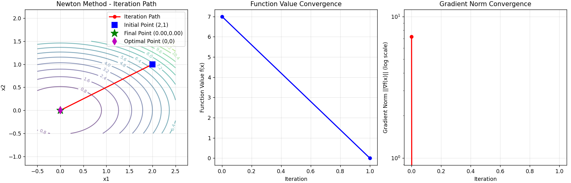
阻尼牛顿法(Damped Newton's Method)
-
原理:牛顿法的改进版本,引入步长控制(通过线搜索确定步长),而不是直接使用牛顿步长。这确保每次迭代都减少目标函数值,提高稳定性。
-
优点:比标准牛顿法更鲁棒,能处理Hessian矩阵非正定或初始点远离最小值的情况。
-
缺点:仍需要计算Hessian矩阵,计算成本较高。
核心公式
-
牛顿方向:
-
带步长的迭代:
-
步长通过线搜索确定:
与标准牛顿法的区别
增加了步长控制机制,确保
变尺度法(拟牛顿法)
DFP(Davidon-Fletcher-Powell)
-
原理:一种拟牛顿法,通过迭代更新近似Hessian逆矩阵(而不是直接计算),满足割线条件(即近似矩阵与梯度变化一致)。DFP使用秩二更新公式。
-
优点:避免计算Hessian矩阵,计算效率较高;收敛速度超线性。
-
缺点:数值稳定性较差,可能受舍入误差影响;在实践中已被BFGS取代。
核心公式
-
拟牛顿方向:
-
DFP更新公式:
其中:
算法步骤
-
初始
-
计算方向
-
线搜索求
-
计算
-
按DFP公式更新
BFGS(Broyden-Fletcher-Goldfarb-Shanno)
-
原理:另一种拟牛顿法,同样通过更新近似Hessian逆矩阵(或Hessian矩阵)来模拟牛顿法。BFGS使用不同的秩二更新公式,通常比DFP更稳定。
-
优点:数值稳定性好,收敛速度快(超线性),无需计算二阶导数,是当前最流行的拟牛顿法。
-
缺点:需要存储近似矩阵,内存需求随问题规模增大而增加。
核心公式
- 拟牛顿方向:
- BFGS更新公式:
等价形式(更常用):
其中:
算法步骤
-
初始
-
计算方向
-
线搜索求
-
计算
-
按BFGS公式更新